4  Policy Gradient and Actor-Critic Methods

\[ \newcommand{\E}{\mathbb{E}} \newcommand{\R}{\mathbb{R}} \newcommand{\Prob}{\mathbb{P}} \newcommand{\BR}{\operatorname{BR}} \newcommand{\eps}{\varepsilon} \newcommand{\given}{\,\vert\,} \newcommand{\argmax}{\operatorname*{arg\,max}} \newcommand{\argmin}{\operatorname*{arg\,min}} \newcommand{\sm}{\setminus} \newcommand{\defeq}{\equiv} \]

Every algorithm so far has parameterized a value and read a policy off it. Chapter 3 ended by replacing the table of values with a function \(\hat{v}(s,w)\) or \(\hat{q}(s,a,w)\), but the decision rule was still whatever \(\argmax_{a}\hat{q}(s,a,w)\) happened to be. This chapter parameterizes the policy itself, \(\pi(a\given s,\theta)\), and pushes \(\theta\) uphill on the value it delivers. That is a different kind of algorithm: the object being learned is the thing you act with, not an intermediate quantity you act on. It is also the family used to post-train large language models, which is the main reason it matters outside a lecture room.

NoteSource:

Ben Moll’s RL lecture slides, Lecture 4.

4.1 From value-based to policy-based methods

Why the shift

Chapters 1 to 3 are all value-based. They estimate \(v_{\pi}\) or \(q_{\pi}\), and the policy is a by-product: greedy or \(\eps\)-greedy with respect to the estimate, as in Definition 2.2. Policy gradient methods are policy-based. They write down a family of policies indexed by \(\theta\), define a scalar measure of how good a policy is, and do gradient ascent on it. In the language of Chapter 1, this is a different way of doing step 2 of Howard policy iteration, the improvement step: instead of re-solving an \(\argmax\) from scratch each round, nudge the current policy in the direction that raises value. Step 1, policy evaluation, is still done by estimating an action-value function, so nothing from Chapters 2 and 3 is thrown away. It gets repurposed.

NoteWhy these are the methods people actually run

Policy gradient methods dominate practice, and most visibly in the post-training of large language models: reinforcement learning from human feedback (RLHF) and reinforcement learning with verifiable rewards (RLVR), the recipe behind reasoning models, are both policy gradient. The reason is structural. A language model is already a parameterized stochastic policy: given a context \(s\), it emits a distribution over next tokens \(a\). There is no table of \(q\)-values to take an \(\argmax\) over, and no sensible way to build one. What there is, is a differentiable \(\pi(a\given s,\theta)\) with billions of parameters and a reward signal at the end of a generated sequence. That is exactly the setting the theorems below are written for. The standard workhorse algorithm, proximal policy optimization (PPO), is a refinement of the plain gradient step derived in this chapter.

Policies as tables, policies as functions

Until now a policy has been a table. With nine states and five actions it is a \(9\times5\) grid whose \((s,a)\) cell holds \(\pi(a\given s)\), one number per state-action pair, read by lookup and written by assignment.

Replace it with a parameterized function

\[ \pi(a\given s,\theta),\qquad \theta\in\R^{m}, \tag{4.1}\]

where \(\theta\) might be the weights of a neural network whose input is \(s\) and whose outputs are the probabilities of each action. This is the same move Chapter 3 made for values in Equation 3.11, and it buys the same two things for the same two reasons:

  1. Storage. The table has \(|\mathcal{S}|\times|\mathcal{A}|\) entries. The function has \(m\) parameters, and \(m\) can be far smaller.
  2. Generalization. Changing one cell of a table changes the policy at one state. Changing \(\theta\) moves \(\pi\) at many states at once, so experience at \(s\) informs behaviour at states never visited.
Tip

The parallel with Equation 3.11 is exact, and it is worth being precise about what is not parallel. Equation 3.11 approximates a function, \(v_{\pi}\), that exists independently of the approximation: there is a true \(v_{\pi}\) and \(\hat{v}(s,w)\) is a fit to it. Equation 4.1 is not a fit to anything. There is no “true \(\pi\)” being approximated; the parameterized family simply is the set of policies under consideration, and the optimum is the best member of that family. Function approximation for values introduces approximation error. Policy parameterization introduces a restricted feasible set.

Notation varies: \(\pi(a\given s,\theta)\), \(\pi(a,s,\theta)\), and \(\pi_{\theta}(a\given s)\) all appear in the literature and all mean the same object. This chapter uses the first. For the deterministic case of the next section the policy returns an action rather than a distribution, and is written \(a=\pi(s,\theta)\).

4.2 Setting up the optimization

The goal is to choose \(\theta\) to maximize

\[ v_{\pi}(s)=\E_{0}\!\left[\sum_{t=0}^{\infty}\gamma^{t}r(s_{t},a_{t})\ \given\ s_{0}=s\right], \qquad s_{t+1}\sim p(\cdot\given s_{t},a_{t}),\ \ a_{t}\sim\pi(\cdot\given s_{t},\theta), \]

by some version of gradient ascent,

\[ \theta_{j+1}=\theta_{j}+\alpha\,\nabla_{\theta}J(\theta_{j}), \tag{4.2}\]

ascent rather than descent because the problem is a maximization. In practice the true gradient is unavailable and Equation 4.2 is run in its stochastic form, which is Equation 2.13 with the sign flipped: whenever the gradient can be written \(\nabla_{\theta}J(\theta)=\E[\text{something}(\theta)]\), a single sampled realization of that something is a legitimate step direction. That “whenever” is the entire technical content of this chapter.

Two problems stand between here and there.

Problem 1: \(v_{\pi}\) is not a scalar

\(v_{\pi}(s)\) is defined for every \(s\in\mathcal{S}\), so it is a vector of length \(|\mathcal{S}|\), or a function when the state space is continuous. Gradient ascent maximizes a number. There is nothing to ascend on until the vector is collapsed to a scalar.

The collapse is a weighted average across states:

\[ J(\theta)=\sum_{s\in\mathcal{S}}v_{\pi}(s)\,\mu(s), \tag{4.3}\]

where \(\mu\) is some distribution over starting states, for instance uniform. Read Equation 4.3 as expected value under a random initial state: \(J(\theta)=\E_{s_{0}\sim\mu}[v_{\pi}(s_{0})]\). The choice of \(\mu\) matters for which policy is optimal, since it says which states you care about doing well in, but it is exogenous and does not depend on \(\theta\), which is what makes it harmless to differentiate through.

Problem 2: the model reappears

With a scalar objective in hand, differentiate. Take the deterministic case \(a=\pi(s,\theta)\) for a moment, since it makes the difficulty most visible, and start from the Bellman equation for \(v_{\pi}\):

\[ v_{\pi}(s)=r\big(s,\pi(s,\theta)\big)+\gamma\sum_{s'\in\mathcal{S}}v_{\pi}(s')\,p\big(s'\given s,\pi(s,\theta)\big). \]

The parameter \(\theta\) enters through the action, and the action enters both the reward function and the transition density. So the chain rule produces

\[ \nabla_{\theta}v_{\pi}(s)=\Big(\underbrace{\nabla_{a}r(s,\pi)}_{\text{unknown}}+\gamma\sum_{s'\in\mathcal{S}}v_{\pi}(s')\underbrace{\nabla_{a}p(s'\given s,\pi)}_{\text{unknown}}\Big)\nabla_{\theta}\pi+\gamma\sum_{s'\in\mathcal{S}}\big(\nabla_{\theta}v_{\pi}(s')\big)\,p(s'\given s,\pi). \tag{4.4}\]

Both marked terms require the model: how the reward responds to a marginal change in the action, and how the transition density does. Neither is available in a model-free setting.

Important

This is the same obstruction, in a new place. Chapter 2 met it in the policy improvement step, \(\argmax_{\pi}\{\mathbf{r}_{\pi}+\gamma\mathbf{P}_{\pi}\mathbf{v}\}\), which reads the model to turn a value into a decision, and solved it by working with action values instead: Equation 2.6 is an expectation, and expectations can be sampled. Here the same \((\mathbf{r},\mathbf{P})\) blocks the gradient rather than the maximization. The resolution is the same, and it is called the policy gradient theorem: rewrite \(\nabla_{\theta}J\) so that the model-dependent pieces are absorbed into \(q_{\pi}\), which can be estimated from samples.

Two versions follow. The deterministic one is more pedagogical and came later historically; the stochastic one is the version implemented in practice and is what people mean by “the policy gradient theorem”.

4.3 The deterministic policy gradient theorem

Theorem 4.1 (Deterministic policy gradient theorem) Let \(\mathcal{S}\) be finite, let \(\gamma\in(0,1)\), let the policy be deterministic, \(a=\pi(s,\theta)\) and differentiable in \(\theta\), and let \(J(\theta)=\sum_{s}v_{\pi}(s)\mu(s)\) as in Equation 4.3. Then

\[ \nabla_{\theta}J(\theta)=\E_{0}\!\left[\sum_{t=0}^{\infty}\gamma^{t}\,\nabla_{a}q_{\pi}(s_{t},a_{t})\,\nabla_{\theta}\pi(s_{t},\theta)\right], \tag{4.5}\]

where the expectation is over trajectories with \(s_{0}\sim\mu\), \(a_{t}=\pi(s_{t},\theta)\), and \(s_{t+1}\sim p(\cdot\given s_{t},a_{t})\).

Read the hypotheses back in words. The policy is a deterministic function of the state, so the action space must be continuous for \(\nabla_{a}\) to mean anything. The expectation is taken along trajectories generated by the policy being differentiated, so the theorem is a statement about on-policy data in the sense of Definition 3.3. And the model has vanished from the right-hand side entirely: the only unknowns are \(q_{\pi}\) and its derivative in the action, both properties of the value function rather than of the environment. The result is due to Silver et al. (2014).

Step 1: differentiate the Bellman equation. This is Equation 4.4, restated: \[ \nabla_{\theta}v_{\pi}(s)=\Big(\nabla_{a}r(s,\pi)+\gamma\sum_{s'\in\mathcal{S}}v_{\pi}(s')\nabla_{a}p(s'\given s,\pi)\Big)\nabla_{\theta}\pi+\gamma\sum_{s'\in\mathcal{S}}\big(\nabla_{\theta}v_{\pi}(s')\big)p(s'\given s,\pi). \] The first group collects the effect of \(\theta\) on today’s action; the second collects its effect on the continuation value, because \(v_{\pi}\) at every future state also depends on \(\theta\).

Step 2: recognize the bracket as \(\nabla_{a}q_{\pi}\). The action value under \(\pi\) is, by Equation 2.5, \[ q_{\pi}(s,a)=r(s,a)+\gamma\sum_{s'\in\mathcal{S}}v_{\pi}(s')\,p(s'\given s,a). \] Differentiate it with respect to \(a\), holding the continuation values \(v_{\pi}(s')\) fixed, which is legitimate because \(q_{\pi}(s,a)\) is by construction the value of deviating to \(a\) today only and following \(\pi\) from tomorrow on: \[ \nabla_{a}q_{\pi}(s,a)=\nabla_{a}r(s,a)+\gamma\sum_{s'\in\mathcal{S}}v_{\pi}(s')\,\nabla_{a}p(s'\given s,a). \] That is exactly the bracket in Step 1. Substituting, \[ \nabla_{\theta}v_{\pi}(s)=\nabla_{a}q_{\pi}\big(s,\pi(s,\theta)\big)\,\nabla_{\theta}\pi(s,\theta)+\gamma\sum_{s'\in\mathcal{S}}\big(\nabla_{\theta}v_{\pi}(s')\big)\,p\big(s'\given s,\pi(s,\theta)\big). \tag{4.6}\] The two unknown model derivatives have been packed into one object, \(\nabla_{a}q_{\pi}\), and both instances of the model that remain, \(p(s'\given s,\pi)\), sit where a Bellman equation always puts them.

Step 3: read Equation 4.6 as a Bellman equation. Define the unknown function \(x(s)\defeq\nabla_{\theta}v_{\pi}(s)\) and the “reward” \[ \rho(s)\defeq\nabla_{a}q_{\pi}\big(s,\pi(s,\theta)\big)\,\nabla_{\theta}\pi(s,\theta). \] Both are functions of the state alone, since \(\theta\) is fixed while we differentiate. Then Equation 4.6 reads \[ x(s)=\rho(s)+\gamma\sum_{s'\in\mathcal{S}}x(s')\,p_{\pi}(s'\given s), \] which is Equation 1.2, the Bellman equation of a Markov reward process in the sense of Definition 1.1, with reward \(\rho\) and transition kernel \(p_{\pi}\). Nothing about Definition 1.1 requires the reward to be a scalar: run the argument coordinate by coordinate on the \(m\) components of \(x\) and \(\rho\) and it goes through unchanged.

Step 4: solve it as a present discounted value. In matrix form, \(\mathbf{x}=\boldsymbol{\rho}+\gamma\mathbf{P}_{\pi}\mathbf{x}\). Since \(\mathbf{P}_{\pi}\) is row-stochastic its spectral radius is \(1\), so for \(\gamma\in(0,1)\) the matrix \(I-\gamma\mathbf{P}_{\pi}\) is invertible and the solution is unique: \[ \mathbf{x}=(I-\gamma\mathbf{P}_{\pi})^{-1}\boldsymbol{\rho}=\sum_{t=0}^{\infty}\gamma^{t}\mathbf{P}_{\pi}^{t}\boldsymbol{\rho}, \] the Neumann series converging because \(\|\gamma\mathbf{P}_{\pi}\|<1\). Row \(s\) of \(\mathbf{P}_{\pi}^{t}\boldsymbol{\rho}\) is \(\E[\rho(s_{t})\given s_{0}=s]\), so component-wise this says \[ \nabla_{\theta}v_{\pi}(s_{0})=\E_{0}\!\left[\sum_{t=0}^{\infty}\gamma^{t}\,\nabla_{a}q_{\pi}(s_{t},a_{t})\,\nabla_{\theta}\pi(s_{t},\theta)\right], \qquad a_{t}=\pi(s_{t},\theta),\ \ s_{t+1}\sim p(\cdot\given s_{t},a_{t}). \]

Step 5: average over starting states. By Equation 4.3, \(\nabla_{\theta}J(\theta)=\sum_{s}\mu(s)\nabla_{\theta}v_{\pi}(s)\), since \(\mu\) does not depend on \(\theta\). Drawing \(s_{0}\sim\mu\) instead of fixing it gives Equation 4.5. \(\square\)

TipWhat the proof actually did

Three moves, and only the middle one is specific to this problem. Differentiate the Bellman equation. Notice that the awkward terms are precisely the derivative of \(q_{\pi}\) in the action. Then observe that what is left is itself a Bellman equation, in the new unknown \(\nabla_{\theta}v_{\pi}\), and therefore has the standard present-discounted-value solution.

The last step is where the model-free property is won. The gradient of the value at \(s_{0}\) is a discounted sum of local quantities along a trajectory, and a trajectory is something you can sample. You do not need \(p\) to compute the sum; you need \(p\) only to generate the states, which the environment does for free.

Turning Equation 4.5 into an algorithm is mechanical. It has the form \(\nabla_{\theta}J(\theta)=\E[\text{something}(\theta)]\), so replacing the expectation by one sampled trajectory of length \(T\) gives the stochastic gradient ascent step

\[ \theta_{j+1}=\theta_{j}+\alpha\sum_{t=0}^{T}\gamma^{t}\,\nabla_{a}q_{\pi}(s_{t},a_{t})\,\nabla_{\theta}\pi(s_{t},\theta_{j}). \]

Which leaves one thing outstanding: an estimate of \(q_{\pi}\), and of its derivative \(\nabla_{a}q_{\pi}\). Hold that thought.

4.4 The stochastic policy gradient theorem

Now let the policy be stochastic, \(a_{t}\sim\pi(\cdot\given s_{t},\theta)\).

Theorem 4.2 (Stochastic policy gradient theorem) Let \(\mathcal{S}\) and \(\mathcal{A}\) be finite, let \(\gamma\in(0,1)\), let \(\pi(a\given s,\theta)>0\) be differentiable in \(\theta\) for all \((s,a)\), and let \(J(\theta)=\sum_{s}v_{\pi}(s)\mu(s)\) as in Equation 4.3. Then

\[ \nabla_{\theta}J(\theta)=\E_{0}\!\left[\sum_{t=0}^{\infty}\gamma^{t}\,q_{\pi}(s_{t},a_{t})\,\nabla_{\theta}\ln\pi(a_{t}\given s_{t},\theta)\right], \tag{4.7}\]

where the expectation is over trajectories with \(s_{0}\sim\mu\), \(a_{t}\sim\pi(\cdot\given s_{t},\theta)\), and \(s_{t+1}\sim p(\cdot\given s_{t},a_{t})\).

Compare the hypotheses with Theorem 4.1. Positivity of \(\pi\) is new and is needed for \(\ln\pi\) to be defined; differentiability in \(\theta\) replaces differentiability in \(a\), so the action space may now be finite. Compare the conclusions: \(\nabla_{a}q_{\pi}\) has become plain \(q_{\pi}\), and \(\nabla_{\theta}\pi\) has become \(\nabla_{\theta}\ln\pi\). Both changes come from a single algebraic step in the proof.

Step 1: differentiate the Bellman equation. For a fixed stochastic policy \(\pi\), Equation 2.1 without the maximization reads \[ v_{\pi}(s)=\sum_{a\in\mathcal{A}}\pi(a\given s,\theta)\left(r(s,a)+\gamma\sum_{s'\in\mathcal{S}}v_{\pi}(s')\,p(s'\given s,a)\right). \] Differentiate with respect to \(\theta\) by the product rule. Note what has changed relative to the deterministic case: \(\theta\) now enters only through \(\pi\), because \(r(s,a)\) and \(p(s'\given s,a)\) are evaluated at fixed actions \(a\) that are summed over, not at a \(\theta\)-dependent action. So no \(\nabla_{a}r\) or \(\nabla_{a}p\) can arise: \[ \nabla_{\theta}v_{\pi}(s)=\sum_{a\in\mathcal{A}}\nabla_{\theta}\pi(a\given s,\theta)\left(r(s,a)+\gamma\sum_{s'}v_{\pi}(s')p(s'\given s,a)\right)+\sum_{a\in\mathcal{A}}\pi(a\given s,\theta)\,\gamma\sum_{s'}\big(\nabla_{\theta}v_{\pi}(s')\big)p(s'\given s,a). \]

Step 2: name the bracket. By Equation 2.5 the bracket is \(q_{\pi}(s,a)\), so \[ \nabla_{\theta}v_{\pi}(s)=\sum_{a\in\mathcal{A}}\nabla_{\theta}\pi(a\given s,\theta)\,q_{\pi}(s,a)+\gamma\sum_{a\in\mathcal{A}}\pi(a\given s,\theta)\sum_{s'\in\mathcal{S}}\big(\nabla_{\theta}v_{\pi}(s')\big)p(s'\given s,a). \] The second term is already in Bellman form: it averages \(\nabla_{\theta}v_{\pi}(s')\) against \(\pi\) and then against \(p\), which is exactly the policy-averaged transition \(p_{\pi}\) of Definition 2.1. The first term is not, because its weights are \(\nabla_{\theta}\pi(a\given s,\theta)\) rather than \(\pi(a\given s,\theta)\).

Step 3: the log trick. Multiply and divide by \(\pi\), which is legitimate because \(\pi>0\): \[ \nabla_{\theta}\pi(a\given s,\theta)=\pi(a\given s,\theta)\,\frac{\nabla_{\theta}\pi(a\given s,\theta)}{\pi(a\given s,\theta)}=\pi(a\given s,\theta)\,\nabla_{\theta}\ln\pi(a\given s,\theta), \tag{4.8}\] the second equality being the chain rule for \(\ln\). Substituting, both terms now carry the same weights \(\pi(a\given s,\theta)\) and can be collected: \[ \nabla_{\theta}v_{\pi}(s)=\sum_{a\in\mathcal{A}}\pi(a\given s,\theta)\left(\nabla_{\theta}\ln\pi(a\given s,\theta)\,q_{\pi}(s,a)+\gamma\sum_{s'\in\mathcal{S}}\big(\nabla_{\theta}v_{\pi}(s')\big)p(s'\given s,a)\right). \tag{4.9}\]

Step 4: read it as a Bellman equation and solve. Equation 4.9 has exactly the shape of the stochastic-policy Bellman equation, with unknown \(x(s)=\nabla_{\theta}v_{\pi}(s)\) and state-action reward \[ \rho(s,a)\defeq q_{\pi}(s,a)\,\nabla_{\theta}\ln\pi(a\given s,\theta). \] As in Step 4 of the deterministic proof, \(I-\gamma\mathbf{P}_{\pi}\) is invertible for \(\gamma\in(0,1)\) because \(\mathbf{P}_{\pi}\) is row-stochastic, so the fixed point is unique and equals its present discounted value: \[ \nabla_{\theta}v_{\pi}(s_{0})=\E_{0}\!\left[\sum_{t=0}^{\infty}\gamma^{t}\,q_{\pi}(s_{t},a_{t})\,\nabla_{\theta}\ln\pi(a_{t}\given s_{t},\theta)\right],\qquad a_{t}\sim\pi(\cdot\given s_{t},\theta). \]

Step 5: average over starting states. Drawing \(s_{0}\sim\mu\) in Equation 4.3 gives Equation 4.7. \(\square\)

Why the log trick is the whole point

Equation 4.8 looks like a triviality. It is the step that makes the theorem usable, and the reason is worth spelling out.

Before the trick, the first term of Step 2 is \(\sum_{a}\nabla_{\theta}\pi(a\given s,\theta)\,q_{\pi}(s,a)\): a weighted sum whose weights are gradient components. Those weights are not probabilities. They can be negative, and in fact they sum to zero, since differentiating \(\sum_{a}\pi(a\given s,\theta)=1\) gives \(\sum_{a}\nabla_{\theta}\pi(a\given s,\theta)=0\). There is no distribution you could draw an action from to make that sum an average, so there is no Monte-Carlo estimator for it.

After the trick, the weights are \(\pi(a\given s,\theta)\): the distribution the agent is already sampling from every time it acts. The sum becomes a genuine expectation, and the whole right-hand side of Equation 4.7 becomes an expectation over trajectories the agent generates in the ordinary course of running. Chapter 1’s founding observation then applies verbatim: an expectation you cannot integrate is an expectation you can average.

Tip

Put differently, the log trick moves the derivative off the measure and onto the integrand. The quantity \(\nabla_{\theta}\ln\pi(a\given s,\theta)\), the score, is just another function of \((s,a)\) that you evaluate at the sampled pair, and \(\pi\) is left where it belongs, as the thing generating the sample. This is why the same device shows up under different names across statistics: it is the score-function identity behind maximum likelihood, and the likelihood-ratio estimator in simulation.

The one price is the hypothesis \(\pi>0\). A parameterization that could assign probability zero to an action would make \(\ln\pi\) undefined exactly where it is needed. The standard fix builds positivity into the functional form.

Example 4.1 (Softmax parameterization) Let \(h(s,a,\theta)\) be an arbitrary differentiable preference function, for example the output of a neural network, and set \[ \pi(a\given s,\theta)=\frac{e^{h(s,a,\theta)}}{\sum_{a'\in\mathcal{A}}e^{h(s,a',\theta)}}. \tag{4.10}\] Because the exponential is strictly positive, \(\pi(a\given s,\theta)\in(0,1)\) for every \((s,a)\) and \(\sum_{a}\pi(a\given s,\theta)=1\) automatically. The score has a clean form: \[ \nabla_{\theta}\ln\pi(a\given s,\theta)=\nabla_{\theta}h(s,a,\theta)-\sum_{a'\in\mathcal{A}}\pi(a'\given s,\theta)\,\nabla_{\theta}h(s,a',\theta), \] the gradient of the chosen action’s preference minus its average across actions. Raising \(\theta\) along this direction raises \(h\) for the action taken relative to the others, which is what “make good actions more likely” means concretely. In a network implementation this is simply a softmax output layer.

Important

Softmax settles the exploration problem without any of Chapter 2’s machinery. Definition 2.2 kept every action alive by mixing a greedy policy with a uniform one, an external patch on a policy that would otherwise be degenerate. Under Equation 4.10 every action has strictly positive probability by construction, at every state, for every \(\theta\). Exploration is a property of the parameterization rather than something bolted on afterwards, and it anneals on its own: as the preferences separate, the policy becomes nearly deterministic where it is confident and stays diffuse where it is not.

Comparing the two theorems

Table 4.1: The two policy gradient theorems. They differ in one requirement, and that requirement decides which one gets implemented.
Deterministic, Theorem 4.1 Stochastic, Theorem 4.2
Policy \(a=\pi(s,\theta)\), an action \(a\sim\pi(\cdot\given s,\theta)\), a distribution
Gradient \(\E_{0}\big[\sum_{t}\gamma^{t}\nabla_{a}q_{\pi}(s_{t},a_{t})\nabla_{\theta}\pi(s_{t},\theta)\big]\) \(\E_{0}\big[\sum_{t}\gamma^{t}q_{\pi}(s_{t},a_{t})\nabla_{\theta}\ln\pi(a_{t}\given s_{t},\theta)\big]\)
Needs estimated \(q_{\pi}\) and its action-derivative \(\nabla_{a}q_{\pi}\) \(q_{\pi}\) only, at visited pairs
Action space continuous, or \(\nabla_{a}\) is meaningless finite or continuous
Exploration none: the policy is a point built in, if \(\pi>0\) as in Equation 4.10
Where the \(\theta\)-derivative sits on the action, hence on \(r\) and \(p\) on \(\pi\) alone, hence never on the model

The decisive row is the third. Estimating \(q_{\pi}(s,a)\) from samples is the problem Chapters 2 and 3 solved three separate ways: Monte-Carlo returns Equation 2.6, Sarsa Equation 3.7, Sarsa with function approximation Equation 3.14. Estimating \(\nabla_{a}q_{\pi}(s,a)\) is strictly harder, and not by a constant factor. A derivative is a difference of nearby values divided by a small number, so any noise in the estimate of \(q_{\pi}\) is amplified; and to know how \(q_{\pi}\) moves in \(a\) you need data at neighbouring actions, which a deterministic policy never generates, since it always plays the same action at a given state. The deterministic version therefore has to import an exploration scheme from outside and a differentiable critic in the action, which is what Deep Deterministic Policy Gradient does.

The stochastic version asks only for \(q_{\pi}(s_{t},a_{t})\) at the state-action pairs actually visited, and generates its own spread of actions for free. That is why Equation 4.7, not Equation 4.5, is what “the policy gradient theorem” refers to, and what everything below builds on.

4.5 REINFORCE

Equation 4.7 is a statement of the form \(\nabla_{\theta}J(\theta)=\E[\text{something}(\theta)]\), so Equation 4.2 in its stochastic form says: sample one trajectory, evaluate the something, step. Truncating at horizon \(T\),

\[ \theta_{j+1}=\theta_{j}+\alpha\sum_{t=0}^{T}\gamma^{t}\,q_{\pi}(s_{t},a_{t})\,\nabla_{\theta}\ln\pi(a_{t}\given s_{t},\theta_{j}). \]

The score \(\nabla_{\theta}\ln\pi(a_{t}\given s_{t},\theta_{j})\) is computable: it is a derivative of a function we chose. The action value \(q_{\pi}(s_{t},a_{t})\) is not. Everything in the rest of this chapter is a choice of what to substitute for it, and the two choices available are the two of Table 3.1.

The first choice is Monte Carlo. By Equation 2.6, \(q_{\pi}(s,a)\) is the expected discounted return from \((s,a)\), so the realized return along the sampled trajectory is an unbiased estimate of it:

\[ G_{t}\defeq\sum_{k=t}^{T}\gamma^{k-t}r_{k+1}. \]

Substituting gives the algorithm.

The code behind Figure 4.2 runs both algorithms on one corridor, set up once for the whole chapter, and calls two helpers it does not itself print. step(s, a) returns the next state, the realized reward, and whether the episode ended, where one action advances along six states and the other goes back against a wall at \(s_{0}\); stepping off the far end pays 10 and ends the episode, every other reward is zero in expectation, and every reward carries \(N(0,3^{2})\) noise. prob_back(theta, s) is the softmax Equation 4.10 evaluated at \(s\). Note this is a different environment from the ledge chain of Chapter 3.

NoteAlgorithm: REINFORCE (Monte-Carlo policy gradient)

Initialize \(\theta_{0}\), a step size \(\alpha>0\), and a discount \(\gamma\in(0,1)\). For each episode \(j=0,1,2,\dots\)

  1. Generate a full episode \(s_{0},a_{0},r_{1},\dots,s_{T},a_{T},r_{T+1}\) by following \(\pi(\cdot\given\cdot,\theta_{j})\), indexing rewards as in Chapter 3 so that \(r_{t+1}\) is the reward for acting at \(t\).
  2. Compute the returns \(G_{t}=\sum_{k=t}^{T}\gamma^{k-t}r_{k+1}\) for \(t=0,\dots,T\).
  3. Update the policy parameter once: \[ \theta_{j+1}=\theta_{j}+\alpha\sum_{t=0}^{T}\gamma^{t}\,G_{t}\,\nabla_{\theta}\ln\pi(a_{t}\given s_{t},\theta_{j}). \tag{4.11}\]

REINFORCE is episodic in the exact sense of Definition 3.1: \(G_{0}\) cannot be formed until the reward at \(T\) has been observed, so \(\theta\) cannot move until the episode is over. That is the same limitation MC Basic had in Chapter 2, arriving now in parameter space rather than in a table.

TipWhat the update does, one term at a time

Write a single term of Equation 4.11 using Equation 4.8 in reverse: \[ \alpha\gamma^{t}G_{t}\nabla_{\theta}\ln\pi(a_{t}\given s_{t},\theta_{j})=\alpha\gamma^{t}\underbrace{\frac{G_{t}}{\pi(a_{t}\given s_{t},\theta_{j})}}_{\text{weight}}\nabla_{\theta}\pi(a_{t}\given s_{t},\theta_{j}), \] which is a gradient-ascent step on the probability \(\pi(a_{t}\given s_{t},\theta)\) itself, with the weight in front. Two readings follow, and together they are the whole intuition for policy gradient.

The weight is proportional to \(G_{t}\): actions that turned out well get their probability pushed up, actions that turned out badly get it pushed down, in proportion to how well. That is exploitation.

The weight is inversely proportional to \(\pi(a_{t}\given s_{t},\theta_{j})\): among two actions with the same return, the one that was unlikely to have been tried gets the larger boost. That is exploration, and it falls out of the log rather than being imposed.

A clarification about the pseudocode

Standard presentations of REINFORCE, in Zhao, in Sutton and Barto, and in Murphy, write the update as a loop over \(t\) inside each episode, which makes it look as though \(\theta\) is being updated at every time step. It is not. Equation 4.11 is one update per episode, and the inner loop is only an efficient way of accumulating its sum.

Write \(\theta_{j}^{t}\) for the running value of the accumulator inside episode \(j\), initialized at \(\theta_{j}^{0}=\theta_{j}\). The inner loop performs \[ \theta_{j}^{t+1}=\theta_{j}^{t}+\alpha\gamma^{t}G_{t}\nabla_{\theta}\ln\pi(a_{t}\given s_{t},\theta_{j}),\qquad t=0,\dots,T. \] The point is the argument of the score: it is \(\theta_{j}\), the parameter that generated the episode, held fixed throughout the loop, and never \(\theta_{j}^{t}\). So every increment is a fixed vector, and unrolling the recursion is just addition: \[ \theta_{j}^{T+1}=\theta_{j}^{0}+\alpha\sum_{t=0}^{T}\gamma^{t}G_{t}\nabla_{\theta}\ln\pi(a_{t}\given s_{t},\theta_{j})=\theta_{j+1}, \] which is Equation 4.11. One episode in, one parameter update out.

WarningWhere implementations depart from the theorem

Some implementations genuinely do refresh \(\theta\) inside the loop, evaluating the score at the current running value rather than at \(\theta_{j}\). This is done for sample efficiency, since it extracts several updates from one episode, but it is no longer Equation 4.11: the scores are then evaluated at parameters that have drifted away from the policy which generated the data, so the estimator is biased. Worth knowing which one you are reading.

4.6 The discounted state visitation distribution

Equation 4.7 is an expectation over whole trajectories, with a \(\gamma^{t}\) weight riding on each term. There is an equivalent form that is an expectation over a single state-action pair, and it is the form that licenses incremental algorithms. Getting to it requires one new object.

Definition 4.1 (Discounted state visitation distribution) For a policy \(\pi\) and an initial distribution \(\mu\), define \[ d_{\pi,\mu}(s)\defeq(1-\gamma)\sum_{t=0}^{\infty}\gamma^{t}\,\Prob\big(s_{t}=s\ \given\ s_{0}\sim\mu,\ \pi\big). \tag{4.12}\]

Read Equation 4.12 as: how often the policy is at \(s\), counting a visit at time \(t\) as worth \(\gamma^{t}\), normalized so the weights sum to one. It answers “where does this policy spend its discounted time”, starting from \(\mu\). The factor \((1-\gamma)\) is exactly the normalization that makes it a probability distribution, which is the first thing to verify.

Non-negativity is immediate: every term in Equation 4.12 is a probability times a non-negative weight. It remains to show the entries sum to one, and the cleanest way is the matrix-vector notation of Chapter 1.

Let \(\mathbf{P}_{\pi}\) be the \(n\times n\) policy-averaged transition matrix built from Definition 2.1, with \((\mathbf{P}_{\pi})_{ij}=p_{\pi}(s_{j}\given s_{i})\), and let \(\boldsymbol{\mu}\) be the column vector of initial probabilities. If \(\boldsymbol{\mu}_{t}\) denotes the distribution of \(s_{t}\) as a column vector, then \[ \boldsymbol{\mu}_{t+1}(j)=\sum_{i}\boldsymbol{\mu}_{t}(i)\,(\mathbf{P}_{\pi})_{ij} \qquad\Longleftrightarrow\qquad \boldsymbol{\mu}_{t+1}=\mathbf{P}_{\pi}^{\!\top}\boldsymbol{\mu}_{t}, \] so \(\boldsymbol{\mu}_{t}=(\mathbf{P}_{\pi}^{\!\top})^{t}\boldsymbol{\mu}\) and Equation 4.12 is \[ \mathbf{d}_{\pi,\mu}=(1-\gamma)\sum_{t=0}^{\infty}\gamma^{t}\big(\mathbf{P}_{\pi}^{\!\top}\big)^{t}\boldsymbol{\mu}. \] Now sum the entries by taking the inner product with the vector of ones \(\mathbf{1}\): \[ \mathbf{d}_{\pi,\mu}^{\!\top}\mathbf{1}=(1-\gamma)\sum_{t=0}^{\infty}\gamma^{t}\,\boldsymbol{\mu}^{\!\top}\mathbf{P}_{\pi}^{t}\,\mathbf{1}. \] Two facts finish it. First, \(\mathbf{P}_{\pi}\) is row-stochastic, meaning each row is a probability distribution over next states, so \(\mathbf{P}_{\pi}\mathbf{1}=\mathbf{1}\); by induction \(\mathbf{P}_{\pi}^{t}\mathbf{1}=\mathbf{1}\) for every \(t\). Second, \(\boldsymbol{\mu}\) is a distribution, so \(\boldsymbol{\mu}^{\!\top}\mathbf{1}=1\). Hence every term of the sum collapses to \(\gamma^{t}\), and \[ \mathbf{d}_{\pi,\mu}^{\!\top}\mathbf{1}=(1-\gamma)\sum_{t=0}^{\infty}\gamma^{t}=(1-\gamma)\cdot\frac{1}{1-\gamma}=1. \qquad\square \]

Tip

The geometric series is the whole reason \((1-\gamma)\) appears in Equation 4.12. The unnormalized discounted visit counts \(\sum_{t}\gamma^{t}\Prob(s_{t}=s)\) sum to \(1/(1-\gamma)\), the expected discounted horizon length, so dividing by that number, equivalently multiplying by \((1-\gamma)\), is what turns a set of occupancy weights into a distribution. This is also where the \(1/(1-\gamma)\) in Equation 4.13 below comes from: it is the same constant, moved to the other side.

The proof says \(d_{\pi,\mu}\) is a distribution; it does not say which one. Figure 4.1 solves Equation 4.12 exactly on the six-state corridor this chapter uses later and puts the answer beside the two distributions it interpolates between: the initial distribution \(\mu\) it starts from, and the long-run distribution it approaches as \(\gamma\to1\).

Solving the visitation distribution exactly at two discount factors
import matplotlib.pyplot as plt

# --- the same six-state corridor, made continuing ------------------------------
# States s0 -> ... -> s5 as behind @fig-4-reinforce-qac: advancing moves one state right,
# going back moves one left and bumps a wall at s0, and advancing from s5 steps off the
# end. There it ended the episode; here it RESTARTS at s0, which is the continuing
# version of the same corridor and is what gives the chain a long-run distribution for
# d to be compared against. d itself needs no such fix, only the comparison does.
# Nothing below is random: every number is a linear solve, so the figure is exact.
N_S = 6
P_BACK = 0.25  # the softmax @eq-softmax at a preference gap of ln 3 in favour of advancing
GAMMAS = (0.5, 0.95)  # 0.95 is the corridor's own discount factor


def transition_matrix(p_back):
    """P_pi of @def-policy-averaged: row s is the distribution of the next state."""
    P = np.zeros((N_S, N_S))
    for s in range(N_S):
        if s < N_S - 1:
            P[s, s + 1] += 1.0 - p_back
        else:
            P[s, 0] += 1.0 - p_back  # off the far end and back to the start
        P[s, max(s - 1, 0)] += p_back  # the wall at s0
    return P


def visitation(P, mu, gamma):
    """d_{pi,mu} of @eq-dvisit in closed form, not by simulation.

    The vector form d = (1-gamma) sum_t gamma^t (P^T)^t mu is a Neumann series, so the
    whole infinite sum collapses to one linear solve. No sampling, no truncation of the
    tail, no Monte-Carlo error anywhere in the figure.
    """
    return (1.0 - gamma) * np.linalg.solve(np.eye(N_S) - gamma * P.T, mu)


def stationary(P):
    """The undiscounted long-run distribution: the one that solves d = P_pi^T d.

    Stacking those fixed-point equations with the normalization 1^T d = 1 gives an
    overdetermined system with exactly one solution, which least squares returns.
    """
    A = np.vstack([P.T - np.eye(N_S), np.ones(N_S)])
    return np.linalg.lstsq(A, np.r_[np.zeros(N_S), 1.0], rcond=None)[0]


P = transition_matrix(P_BACK)
mu = np.zeros(N_S)
mu[0] = 1.0  # every episode starts at s0
d_inf = stationary(P)
ds = [visitation(P, mu, g) for g in GAMMAS]

# Position along the corridor, so that E[position] summarizes a whole distribution in one
# number and the interpolation from mu to the long run can be drawn as a single curve.
pos = np.arange(N_S)
grid = np.linspace(0.0, 0.995, 400)
sweep = np.array([visitation(P, mu, g) @ pos for g in grid])

series = [(mu, INK), (ds[0], COL["sky"]), (ds[1], COL["blue"]), (d_inf, GREY)]

fig, (axL, axR) = plt.subplots(1, 2, figsize=(9.6, 4.0))
trim(axL), trim(axR)

# --- left: the four distributions over the same six states -------------------
w = 0.2
for k, (v, colour) in enumerate(series):
    axL.bar(pos + (k - 1.5) * w, v, width=w * 0.92, color=colour, zorder=3)
axL.set_xticks(pos)
axL.set_xticklabels([rf"$s_{{{s}}}$" for s in pos])
axL.set_xlim(-0.62, 5.62)
axL.set_ylim(0, 1.15)
axL.set_yticks([0, 0.2, 0.4, 0.6, 0.8, 1.0])
axL.set_xlabel("state")
axL.set_ylabel("probability")
axL.set_title("Discounting tilts the weight toward the states reached first",
              fontsize=11)

# Each label sits above its own bars, in space no bar reaches: the whole upper half of
# the panel is empty except for mu's single spike at s0.
label_at(axL, -0.28, 1.06, r"$\mu$: all mass on $s_{0}$", color=INK, fontsize=9.5)
label_at(axL, 0.02, 0.70, r"$d_{\pi,\mu}$ at $\gamma=0.5$",
         color=COL["sky"], fontsize=9.5)
label_at(axL, 2.15, 0.32, r"$d_{\pi,\mu}$ at $\gamma=0.95$",
         color=COL["blue"], fontsize=9.5)
label_at(axL, 5.45, 0.26, "undiscounted\nlong run", color=GREY, fontsize=9.5,
         ha="right", va="bottom", linespacing=1.35)
label_at(axL, 1.95, 0.94,
         r"$\mathbf{d}_{\pi,\mu}=(1-\gamma)(\mathbf{I}-\gamma"
         r"\mathbf{P}_{\pi}^{\top})^{-1}\boldsymbol{\mu}$, solved exactly;"
         "\nall four series sum to 1",
         color=INK, fontsize=9, va="top", linespacing=1.5)

# --- right: where d lands, as gamma runs the whole way from 0 to 1 -----------
# Only the long-run rule is drawn. The other endpoint is mu, whose mean position is zero,
# so its rule would lie under the axis spine and add ink without adding information.
axR.plot([0, 1], [d_inf @ pos] * 2, color=GREY, lw=0.9, ls="--", zorder=2)
axR.plot(grid, sweep, color=INK, lw=2.0, zorder=4)
for g, (_, colour) in zip(GAMMAS, series[1:3]):
    y = visitation(P, mu, g) @ pos
    axR.plot([g, g], [0, y], color=colour, lw=0.9, ls=":", zorder=3)
    axR.plot([g], [y], "o", color=colour, ms=6, zorder=5)
axR.set_xlim(0, 1.0)
axR.set_ylim(0, 2.75)
axR.set_xticks([0, 0.25, 0.5, 0.75, 1.0])
axR.set_xlabel(r"discount factor $\gamma$")
axR.set_ylabel("mean position along the corridor")
axR.set_title(r"$\gamma$ dials $d_{\pi,\mu}$ from $\mu$ to the long run", fontsize=11)

# Every label sits in the wedge the curve leaves empty: the two endpoint tags at the left
# margin, one above the dashed rule and one above the curve's flat start, and each marked
# gamma beside its own drop line, low enough that the curve is nowhere near.
label_at(axR, 0.02, d_inf @ pos + 0.15, r"$\gamma\to1$: the undiscounted long run",
         color=GREY, fontsize=9)
label_at(axR, 0.03, 0.52, r"$\gamma=0$: $d_{\pi,\mu}=\mu$", color=GREY, fontsize=9)
label_at(axR, 0.53, 0.22, r"$\gamma=0.5$", color=COL["sky"], fontsize=9.5)
label_at(axR, 0.92, 0.80, r"$\gamma=0.95$", color=COL["blue"], fontsize=9.5, ha="right")

fig.tight_layout()

# ponytail: one runnable check of the figure's claims, on the exact numbers plotted. Each
# row is a probability distribution, which is what @def-visitation asserts; the four are
# ordered by first-order stochastic dominance, mu earliest and the long run latest, which
# is the sense in which d sits between them; and d minus the long run changes sign exactly
# once, which is the "more weight early, less weight late" the left title claims.
rows = np.array([mu] + ds + [d_inf])
assert np.allclose(rows.sum(axis=1), 1.0)
assert np.all(np.diff(np.cumsum(rows, axis=1), axis=0) <= 1e-12)
assert all(np.count_nonzero(np.diff(np.sign(d - d_inf))) == 1 for d in ds)
plt.show()
Figure 4.1: The most abstract object in this chapter, drawn. Same six-state corridor as Figure 4.2, held at a fixed policy that advances with probability 0.75 at every state, which is the softmax Equation 4.10 at a preference gap of \(\ln 3\); the one change is that stepping off the far end restarts at \(s_{0}\) instead of ending the episode, which makes the chain continuing and so gives it a long-run distribution for \(d_{\pi,\mu}\) to be measured against. Nothing is simulated: the series in Equation 4.12 is a Neumann series, so it collapses to the single solve \(\mathbf{d}_{\pi,\mu}=(1-\gamma)(\mathbf{I}-\gamma\mathbf{P}_{\pi}^{\top})^{-1}\boldsymbol{\mu}\) and every bar is exact. Left: \(\mu\) is all mass on \(s_{0}\); the undiscounted long run is nearly flat, because a policy that mostly advances and then restarts spends comparable time in all six states; and \(d_{\pi,\mu}\) lies between the two, being a geometric average of the distributions of \(s_{0},s_{1},s_{2},\dots\) with weights \((1-\gamma)\gamma^{t}\). All four sum to one, which is what Definition 4.1 proves. The tilt is that \(\gamma^{t}\) doing its work: a visit at time \(t\) counts \(\gamma^{t}\), so states the policy reaches early carry more weight than the long run gives them and late ones carry less, and the crossover slides down the corridor as \(\gamma\) rises, from between \(s_{1}\) and \(s_{2}\) at \(\gamma=0.5\) to between \(s_{2}\) and \(s_{3}\) at \(\gamma=0.95\). Right: the same statement compressed into one number, the mean position under \(d_{\pi,\mu}\), over the whole range of \(\gamma\). At \(\gamma=0\) only \(t=0\) carries weight and \(d_{\pi,\mu}\) is \(\mu\), the long-run value is reached only in the limit, and at the corridor’s own \(\gamma=0.95\) the mean position is 2.10 against the long run’s 2.32: a discount factor that looks close to one still samples noticeably nearer the start. This is the distribution Equation 4.13 asks the gradient to be an expectation over, and it is not the one an implementation gets by reading states off an ongoing trajectory.

The simple expectation form

Start from the present-discounted-value form Equation 4.7 and exchange the sum and the expectation, which is legitimate by dominated convergence when rewards are bounded and \(\gamma<1\): \[ \nabla_{\theta}J(\theta)=\sum_{t=0}^{\infty}\gamma^{t}\,\E\big[q_{\pi}(s_{t},a_{t})\,\nabla_{\theta}\ln\pi(a_{t}\given s_{t},\theta)\big]. \]

Now write out the time-\(t\) expectation by conditioning first on the state and then on the action. Given \(s_{t}=s\), the action is drawn from \(\pi(\cdot\given s,\theta)\) regardless of \(t\), so \[ \E\big[q_{\pi}(s_{t},a_{t})\nabla_{\theta}\ln\pi(a_{t}\given s_{t},\theta)\big] =\sum_{s\in\mathcal{S}}\Prob(s_{t}=s)\underbrace{\sum_{a\in\mathcal{A}}\pi(a\given s,\theta)\,q_{\pi}(s,a)\,\nabla_{\theta}\ln\pi(a\given s,\theta)}_{\defeq\ g(s)}, \] where \(\Prob(s_{t}=s)\) abbreviates \(\Prob(s_{t}=s\given s_{0}\sim\mu,\pi)\). The crucial observation is that \(g(s)\) does not depend on \(t\): it is a property of the state and the fixed policy only. So \(t\) appears nowhere except in \(\gamma^{t}\) and in \(\Prob(s_{t}=s)\), and the sum over \(t\) can be pushed inside the sum over \(s\): \[ \nabla_{\theta}J(\theta)=\sum_{s\in\mathcal{S}}\underbrace{\left[\sum_{t=0}^{\infty}\gamma^{t}\Prob(s_{t}=s)\right]}_{=\ d_{\pi,\mu}(s)/(1-\gamma)}g(s) =\frac{1}{1-\gamma}\sum_{s\in\mathcal{S}}d_{\pi,\mu}(s)\,g(s), \] the identification of the bracket being Equation 4.12 divided by \((1-\gamma)\). Finally, \(\sum_{s}d_{\pi,\mu}(s)(\cdot)\) is an expectation because Definition 4.1 is a distribution, and \(g(s)\) is itself an expectation over \(a\sim\pi(\cdot\given s,\theta)\). Composing the two gives Equation 4.13. \(\square\)

\[ \nabla_{\theta}J(\theta)=\frac{1}{1-\gamma}\,\E_{s\sim d_{\pi,\mu},\ a\sim\pi(\cdot\given s,\theta)}\big[\,q_{\pi}(s,a)\,\nabla_{\theta}\ln\pi(a\given s,\theta)\,\big]. \tag{4.13}\]

Important

Equation 4.7 and Equation 4.13 are the same number written two ways, and the difference between them is where the discounting lives. In Equation 4.7 it is in the summand, as an explicit \(\gamma^{t}\) attached to each term of a trajectory. In Equation 4.13 it has migrated into the sampling distribution: all the \(\gamma^{t}\) weighting is now inside \(d_{\pi,\mu}\), and what is left outside is a single expectation over one state-action pair.

That is what makes incremental algorithms possible. Estimating Equation 4.7 needs a whole trajectory, because the summand is indexed by \(t\). Estimating Equation 4.13 needs one draw of \((s,a)\), so a single transition already supports a gradient step. REINFORCE is episodic because it targets the first form; actor-critic is incremental because it targets the second.

WarningTwo conveniences hidden in the implementation

The constant \(1/(1-\gamma)\) is never computed. It scales the gradient uniformly, so it is absorbed into the step size \(\alpha\) and disappears. And drawing \(s\) exactly from \(d_{\pi,\mu}\) would require restarting from \(\mu\) and stopping with probability \(1-\gamma\) at each step; implementations instead just use the states encountered along an ongoing trajectory. Both are departures from the theorem as stated, both are standard, and neither is usually flagged.

4.7 Actor-critic methods

What actor and critic mean

Definition 4.2 (Actor and critic) In a policy gradient algorithm, the actor is the policy update, the step that moves \(\theta\) and hence changes what the agent does. The critic is the value estimation that supplies \(q_{\pi}\) to the actor, the step that scores the current policy without changing it.

The names are literal. The actor acts; the critic criticizes, by evaluating what the actor did. Note that this is not a new class of algorithm: actor-critic methods are policy gradient methods, and the terminology names a structure rather than a mechanism. What it emphasizes is that policy-based and value-based learning are running side by side in the same loop, with the value-based part of Chapters 2 and 3 supplying exactly the one quantity Equation 4.13 leaves open.

Which critic

Take the stochastic gradient ascent step implied by Equation 4.13: draw one pair \((s_{t},a_{t})\), absorb the constant into \(\alpha\), and step.

\[ \theta_{t+1}=\theta_{t}+\alpha\,q_{\pi}(s_{t},a_{t})\,\nabla_{\theta}\ln\pi(a_{t}\given s_{t},\theta_{t}). \tag{4.14}\]

Equation 4.14 is the actor, and it is complete except for \(q_{\pi}(s_{t},a_{t})\). There are exactly two ways to get that, and they are the two ways this book has been comparing since Table 1.1:

  • Monte Carlo, substituting the realized return \(G_{t}\). That is REINFORCE, Equation 4.11, and it is episodic.
  • Temporal difference, substituting a bootstrapped estimate maintained by its own recursion. That is actor-critic, and it is incremental.

The step from one to the other is the step from Chapter 2 to Chapter 3, taken a second time, one level up.

The QAC algorithm

The simplest instance keeps a parametric action-value function \(\hat{q}(s,a,w)\) and trains it by Sarsa with function approximation. It is usually called Q actor-critic.

NoteAlgorithm: Q actor-critic (QAC)

Initialize policy parameters \(\theta_{0}\), critic parameters \(w_{0}\), and step sizes \(\alpha_{\theta},\alpha_{w}>0\). At each time step \(t\) of each episode:

  1. Interact. Take \(a_{t}\sim\pi(\cdot\given s_{t},\theta_{t})\), observe \(r_{t+1}\) and \(s_{t+1}\), and draw \(a_{t+1}\sim\pi(\cdot\given s_{t+1},\theta_{t})\).

  2. Critic (value update). \[ w_{t+1}=w_{t}+\alpha_{w}\big[\,r_{t+1}+\gamma\hat{q}(s_{t+1},a_{t+1},w_{t})-\hat{q}(s_{t},a_{t},w_{t})\,\big]\nabla_{w}\hat{q}(s_{t},a_{t},w_{t}). \tag{4.15}\]

  3. Actor (policy update). \[ \theta_{t+1}=\theta_{t}+\alpha_{\theta}\,\hat{q}(s_{t},a_{t},w_{t})\,\nabla_{\theta}\ln\pi(a_{t}\given s_{t},\theta_{t}). \tag{4.16}\]

Two observations make the algorithm intelligible.

The critic is not new. Equation 4.15 is Equation 3.14, character for character: Sarsa with function approximation, the last algorithm of Chapter 3. Its bracket is the TD error of Definition 3.2 in action-value form, and it is multiplied by \(\nabla_{w}\hat{q}\) because the update lands on parameters rather than on a table cell. Nothing about it knows it is serving a policy gradient method.

The actor is Equation 4.14 with the estimate plugged in. The only difference from Equation 4.14 is that the unavailable \(q_{\pi}(s_{t},a_{t})\) has been replaced by the critic’s current guess \(\hat{q}(s_{t},a_{t},w_{t})\).

TipRead the two updates as a division of labour

The critic answers “how good was that?” and the actor answers “then do more of it”. Each supplies the other with what it cannot compute: the actor cannot evaluate its own choices, and the critic has no way to change behaviour. Running them at the same time is what makes the method incremental, since neither has to wait for the other to converge before taking its next step.

Both algorithms on one corridor, scored by the exact objective
def run_reinforce(grid):
    """REINFORCE @eq-reinforce: one full episode in, ONE parameter update out."""
    theta = np.zeros((N_S, 2))
    curve = np.full(len(grid), objective(theta))
    k, steps, n_updates = 1, 0, 0
    while steps < BUDGET:
        s, traj = 0, []
        for _ in range(T_MAX):  # 1. generate a full episode
            p1 = prob_back(theta, s)
            a = 1 if RNG.random() < p1 else 0
            s2, r, done = step(s, a)
            traj.append((s, a, r, p1))
            s = s2
            if done:
                break
        steps += len(traj)
        # The whole episode is scored first, then theta moves once: every score below is
        # evaluated at the theta that generated the episode, per @eq-reinforce. The three
        # lines touching g are the softmax score of @exm-softmax written out by hand for
        # two actions, and g accumulates the entire sum before theta moves at all.
        g, G = np.zeros((N_S, 2)), 0.0  # 2. returns, accumulated backwards
        for t in range(len(traj) - 1, -1, -1):
            s_, a_, r_, p1_ = traj[t]
            G = r_ + GAMMA * G  # G_t, the Monte-Carlo estimate of q_pi(s_t, a_t)
            d = GAMMA**t * G
            g[s_, a_] += d
            g[s_, 0] -= d * (1.0 - p1_)
            g[s_, 1] -= d * p1_
        theta += ALPHA_THETA * g  # 3. ONE update, after the episode
        n_updates += 1
        k = record(curve, k, grid, steps, theta)
    return curve, n_updates


def run_qac(grid):
    """QAC @eq-qac-critic and @eq-qac-actor: one transition in, one update out.

    Not literally the same actor as REINFORCE, in two ways. The estimate of q_pi is the
    critic's q_sa, read BEFORE the critic moves, because @eq-qac-actor asks for
    qhat(s_t, a_t, w_t); and the summand carries no gamma**t, because QAC implements
    @eq-spg-simple, whose discounting has already migrated into d_{pi,mu}. The critic is a
    table q(s,a) = w[s,a], which is @eq-sarsa-fa with indicator features: grad_w qhat is
    then the one-hot vector picking out (s,a), so the update touches that entry alone.
    There is no traj list and no backward pass, because nothing has to be remembered until
    the end, and theta moves inside the transition loop rather than after it.
    """
    theta, w = np.zeros((N_S, 2)), np.zeros((N_S, 2))  # actor table, critic table
    curve = np.full(len(grid), objective(theta))
    k, steps = 1, 0
    while steps < BUDGET:
        s = 0
        p1 = prob_back(theta, s)
        a = 1 if RNG.random() < p1 else 0
        for _ in range(T_MAX):
            s2, r, done = step(s, a)  # 1. interact
            if done:
                target = r
            else:
                p1n = prob_back(theta, s2)
                a2 = 1 if RNG.random() < p1n else 0
                target = r + GAMMA * w[s2, a2]  # bootstrap, not a realized return
            q_sa = w[s, a]
            w[s, a] += ALPHA_W * (target - q_sa)  # 2. critic, @eq-qac-critic
            # The score must be read at the CURRENT theta. Reusing the p1 cached when
            # this state was entered is stale whenever the actor already moved row s,
            # which happens on every wall bump where s2 == s.
            pp = prob_back(theta, s)
            theta[s, a] += ALPHA_THETA * q_sa  # 3. actor, one per transition
            theta[s, 0] -= ALPHA_THETA * q_sa * (1.0 - pp)
            theta[s, 1] -= ALPHA_THETA * q_sa * pp
            steps += 1
            k = record(curve, k, grid, steps, theta)
            if done or steps >= BUDGET:
                break
            s, a, p1 = s2, a2, p1n
    return curve  # its update count is the step count, so there is nothing to report


grid = np.linspace(0, BUDGET, 201)
runs = [run_reinforce(grid) for _ in range(N_RUNS)]
rein, n_up = np.array([c for c, _ in runs]), np.mean([n for _, n in runs])
qac = np.array([run_qac(grid) for _ in range(N_RUNS)])

# ponytail: one runnable check of the figure's central claim, on the simulated runs
# themselves. Per environment step QAC's median must lead over the whole second half of the
# budget, and REINFORCE's spread across runs must be the wider one: faster AND steadier out
# of the same experience, which is what the two estimates of q_pi buy at a common step size.
m_rein, m_qac = np.median(rein, axis=0), np.median(qac, axis=0)
iqr = {k: np.percentile(a, 75, axis=0) - np.percentile(a, 25, axis=0)
       for k, a in (("rein", rein), ("qac", qac))}
half = len(m_qac) // 2
assert np.all(m_qac[half:] > m_rein[half:]), "QAC median does not lead throughout"
assert np.all(iqr["rein"][[half, -1]] > iqr["qac"][[half, -1]]), "REINFORCE not the wider"

fig, ax = new_ax(6.8, 4.6)
j_opt = GAMMA ** (N_S - 1) * R_GOAL
ax.plot([0, BUDGET], [j_opt, j_opt], color=GREY, lw=0.9, ls="--", zorder=2)

for arr, colour in ((rein, COL["sky"]), (qac, COL["vermilion"])):
    lo, med, hi = np.percentile(arr, [25, 50, 75], axis=0)
    ax.fill_between(grid, lo, hi, color=colour, alpha=0.22, lw=0, zorder=3)
    ax.plot(grid, med, color=colour, lw=2.0, zorder=5)

ax.set_xlim(0, BUDGET * 1.02)
ax.set_ylim(2.2, 8.2)  # headroom above the dashed rule carries its tag, not data
ax.set_xticks([0, 5000, 10000, 15000, 20000])
ax.set_xticklabels(["0", "5k", "10k", "15k", "20k"])
ax.set_xlabel("environment steps (transitions consumed)")
ax.set_ylabel(r"$J(\theta)=v_{\pi}(s_{0})$")

# Every label sits in space no curve or band enters: the reference tag above the dashed
# rule, "QAC" in the empty wedge above its own steep rise, "REINFORCE" under its own curve,
# and the two notes in the whole empty lower-right quadrant.
label_at(ax, 300, 7.94, r"$J$ at the optimal policy", color=GREY, fontsize=8.5)
label_at(ax, 3000, 6.95, "QAC", color=COL["vermilion"], fontsize=10.5)
label_at(ax, 6300, 5.25, "REINFORCE", color=COL["sky"], fontsize=10.5)
label_at(ax, 11200, 4.55, f"shaded: interquartile range across {N_RUNS} runs",
         color=GREY, fontsize=8.5, va="top")
label_at(ax, 11200, 3.85,
         "the same 20k transitions buy QAC 20,000\n"
         f"updates and REINFORCE {n_up:,.0f}, one per episode",
         color=INK, fontsize=8.5, va="top")
ax.set_title(r"Same actor, same step size: the estimate of $q_{\pi}$ is the"
             " whole difference", fontsize=11)
plt.show()
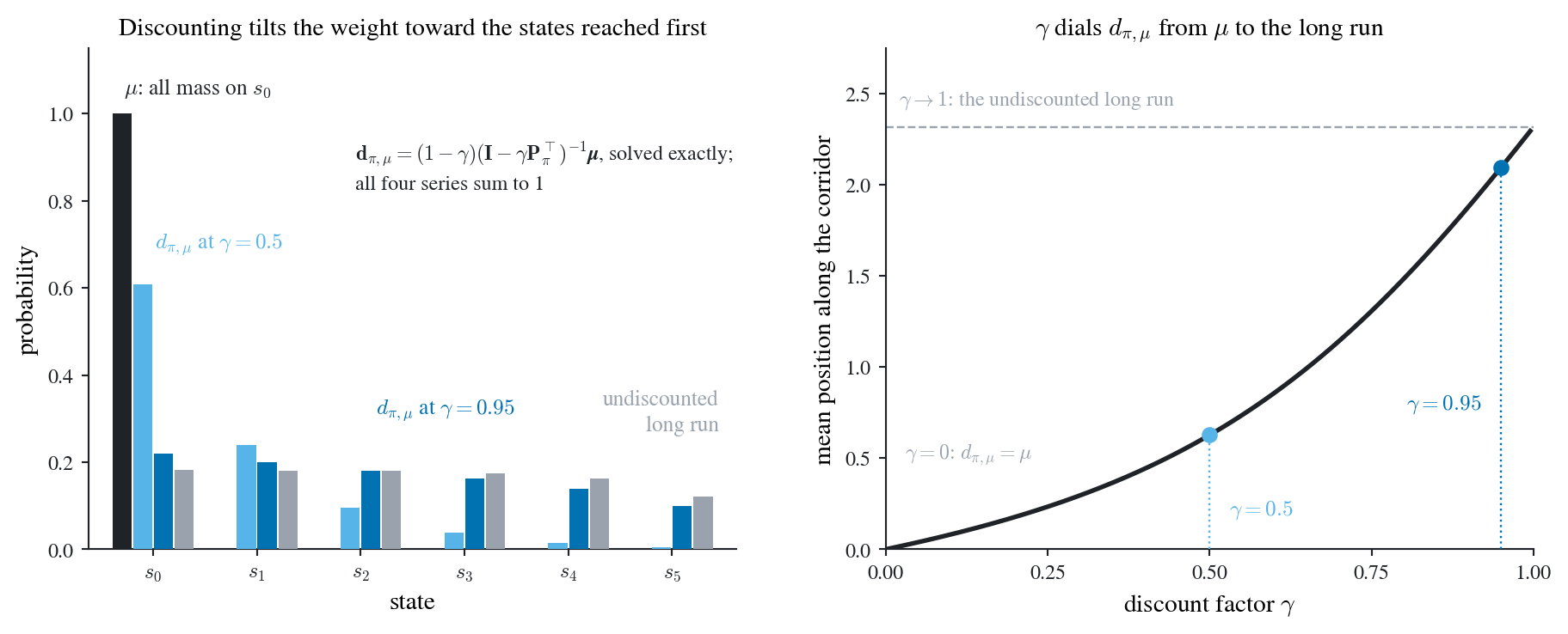
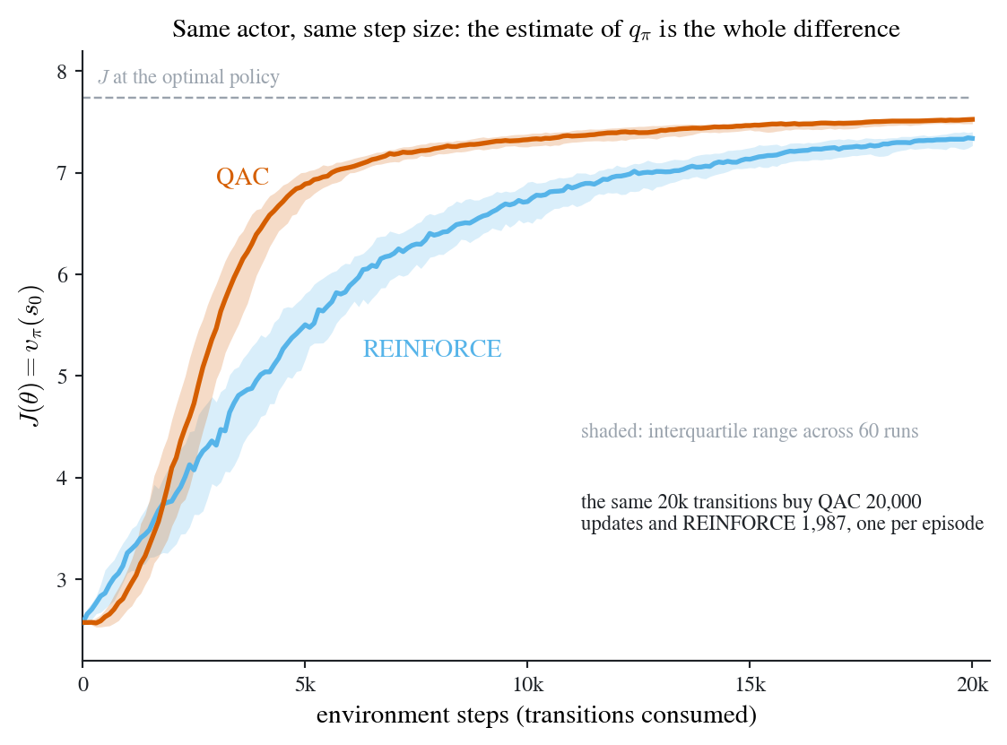
Figure 4.2: REINFORCE Equation 4.11 and QAC Equation 4.16 on the same six-state corridor, charged against environment steps rather than updates. Every episode starts at \(s_{0}\), one action advances along the corridor and one goes back, stepping off the far end pays \(10\) and ends the episode, every other reward is zero in expectation, and every reward carries independent \(N(0,3^{2})\) noise; \(\gamma=0.95\) and episodes are capped at 80 steps. The policy is the softmax Equation 4.10 on a table of preferences, so \(\pi(a\given s,\theta)>0\) everywhere; the critic is a table trained by Equation 3.14 with \(\alpha_{w}=0.05\); and both algorithms use the same actor step size \(\alpha_{\theta}=0.003\), because Equation 4.11 and Equation 4.16 push in the same score direction and the estimate of \(q_{\pi}\) differs. Lines are medians and bands interquartile ranges over 60 runs, with \(J(\theta)=v_{\pi}(s_{0})\) solved for exactly at every point, so the width of a band is dispersion in the learned \(\theta\) rather than measurement noise. QAC sits still for its first thousand steps, since its actor step is scaled by \(\hat{q}\) and the critic starts at zero, and REINFORCE briefly leads. After that the ordering never reverses, for the two reasons of Table 4.2. Timing: 20,000 transitions buy QAC 20,000 parameter updates and REINFORCE about 2,000, one per episode, and by 5,000 steps the median \(J\) is \(6.9\) against \(5.5\). Variance: \(G_{t}\) sums every noisy reward left in the episode while the critic’s target carries one reward plus a bootstrap, so at 10,000 steps REINFORCE’s runs are spread roughly three times as wide. A single run of either would hide that.

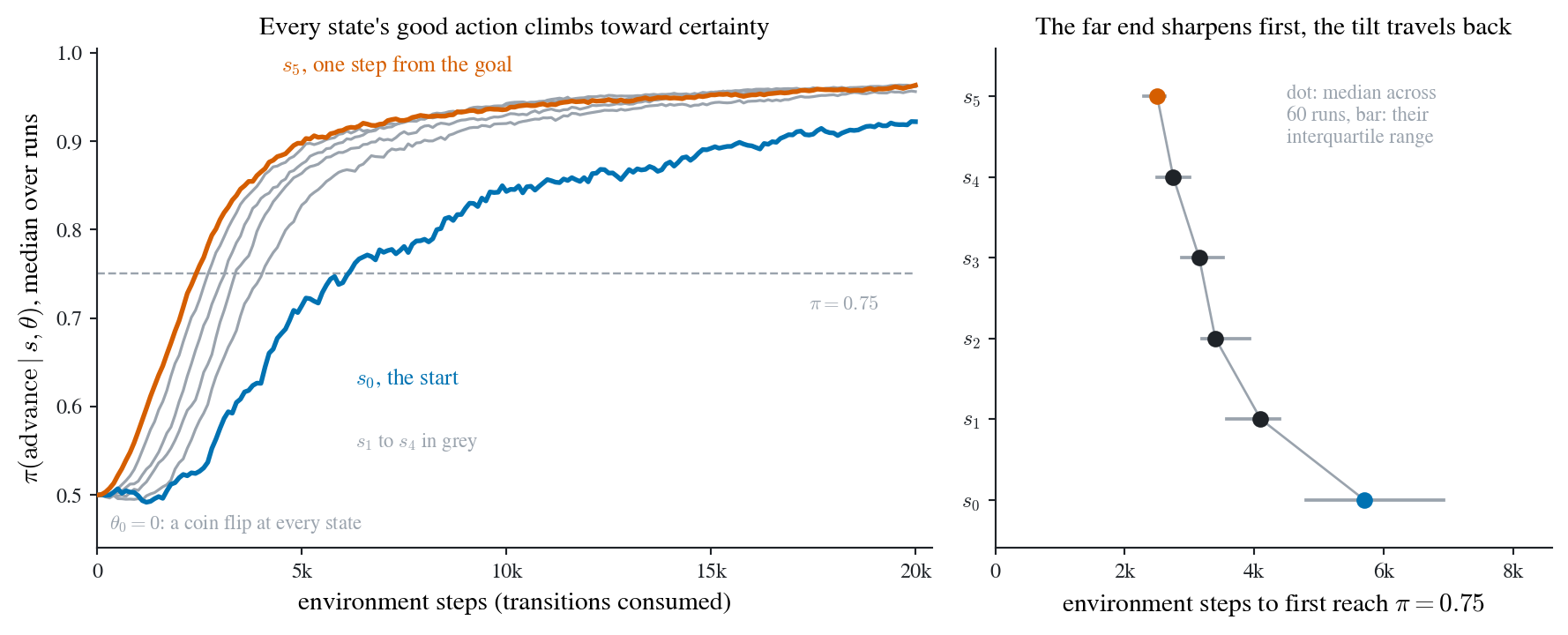
That figure scores QAC by one number per run, \(J(\theta)\) at the start state. Underneath the number is a policy at every state, and Figure 4.3 watches all six of them move, which separates what the actor is doing from what the critic has so far managed to carry back.

Watching the softmax policy sharpen at all six states as QAC ascends
import matplotlib.pyplot as plt

RNG = np.random.default_rng(20260725)

# --- the corridor of @fig-4-reinforce-qac, unchanged --------------------------
# Six states s0 -> ... -> s5. Action 0 ADVANCES, and from s5 it steps off the end,
# collects R_GOAL and ends the episode; action 1 GOES BACK, and at s0 it bumps into
# the wall. Advancing is therefore the good action at every state, which is what makes
# a single probability per state the whole policy worth watching.
N_S, GAMMA, R_GOAL, SD, T_MAX = 6, 0.95, 10.0, 3.0, 80
ALPHA_THETA, ALPHA_W = 0.003, 0.05
BUDGET, N_RUNS, LEVEL = 20_000, 60, 0.75
GRID = np.linspace(0, BUDGET, 201)


def step(s, a):
    """One transition: returns (next state, realized reward, episode over?)."""
    r = RNG.normal(R_GOAL if (a == 0 and s == N_S - 1) else 0.0, SD)
    if a == 0:
        return s + 1, r, s == N_S - 1
    return max(s - 1, 0), r, False


def p_advance(theta):
    """pi(advance | s, theta) at every state: the softmax @eq-softmax, two actions.

    With |A| = 2 the softmax collapses to a logistic in the preference gap, so the
    entire policy is these six numbers and the figure can just plot them.
    """
    return 1.0 / (1.0 + np.exp(theta[:, 1] - theta[:, 0]))


def run_qac():
    """One QAC run; returns pi(advance | s, theta) at every grid point, per state.

    Identical to the QAC of @fig-4-reinforce-qac. What is recorded differs: there the
    run was scored by J(theta), here by the policy itself, sampled on a common grid of
    environment steps and held flat between the crossings of that grid.
    """
    theta, w = np.zeros((N_S, 2)), np.zeros((N_S, 2))
    curve = np.full((len(GRID), N_S), 0.5)  # theta_0 = 0 is a coin flip everywhere
    k, steps = 1, 0
    while steps < BUDGET:
        s = 0
        a = 0 if RNG.random() < p_advance(theta)[s] else 1
        for _ in range(T_MAX):
            s2, r, done = step(s, a)
            if done:
                target = r
            else:
                a2 = 0 if RNG.random() < p_advance(theta)[s2] else 1
                target = r + GAMMA * w[s2, a2]  # bootstrap, not a realized return
            q_sa = w[s, a]  # the critic BEFORE its own update, per @eq-qac-actor
            w[s, a] += ALPHA_W * (target - q_sa)  # critic, @eq-qac-critic
            pa = p_advance(theta)[s]  # the score, read at the CURRENT theta
            theta[s, a] += ALPHA_THETA * q_sa  # actor, @eq-qac-actor
            theta[s, 0] -= ALPHA_THETA * q_sa * pa
            theta[s, 1] -= ALPHA_THETA * q_sa * (1.0 - pa)
            steps += 1
            if k < len(GRID) and GRID[k] <= steps:
                row = p_advance(theta)
                while k < len(GRID) and GRID[k] <= steps:
                    curve[k] = row
                    k += 1
            if done or steps >= BUDGET:
                break
            s, a = s2, a2
    return curve


curves = np.array([run_qac() for _ in range(N_RUNS)])  # runs x grid x state
med = np.median(curves, axis=0)

# When each RUN first puts probability LEVEL on advancing at each state. A run that
# never gets there inside the budget is censored at the budget rather than dropped,
# which understates the lag at s0 instead of hiding it.
hit = curves >= LEVEL
first = np.where(hit.any(axis=1), GRID[hit.argmax(axis=1)], BUDGET)
lo, mid, hi = np.percentile(first, [25, 50, 75], axis=0)

# ponytail: one runnable check of the figure's claim, on the simulated runs themselves.
# The good action must end near certain everywhere without ever reaching one, the fan
# must open in corridor order while it is opening, and the experience each state needs
# to reach LEVEL must fall monotonically as the state gets nearer the goal.
i3k = int(np.argmin(np.abs(GRID - 3000)))
assert 0.85 < med[-1].min() and med[-1].max() < 1.0, np.round(med[-1], 3)
assert np.all(np.diff(med[i3k]) > 0), np.round(med[i3k], 3)
assert np.all(np.diff(mid) < 0), mid

fig, (axL, axR) = plt.subplots(1, 2, figsize=(9.4, 3.9),
                               gridspec_kw={"width_ratios": [1.5, 1]})
trim(axL), trim(axR)

# --- left: the six probabilities, from a coin flip toward one ----------------
# s5 touches the reward and s0 is where J is measured, so those two carry colour and
# the four in between stay grey: the fan's ordering is the right panel's job.
axL.plot([0, BUDGET], [LEVEL, LEVEL], color=GREY, lw=0.9, ls="--", zorder=2)
for j in range(N_S):
    colour = COL["vermilion"] if j == N_S - 1 else COL["blue"] if j == 0 else GREY
    axL.plot(GRID, med[:, j], color=colour, lw=2.0 if colour != GREY else 1.2,
             zorder=5 if colour != GREY else 3)

axL.set_xlim(0, BUDGET * 1.02)
axL.set_ylim(0.44, 1.005)
axL.set_xticks([0, 5000, 10000, 15000, 20000])
axL.set_xticklabels(["0", "5k", "10k", "15k", "20k"])
axL.set_yticks([0.5, 0.6, 0.7, 0.8, 0.9, 1.0])
axL.set_xlabel("environment steps (transitions consumed)")
axL.set_ylabel(r"$\pi(\mathrm{advance}\mid s,\theta)$, median over runs")

# Every label sits where no curve goes: the threshold tag on the dashed rule at the
# right margin, the s5 tag in the empty strip above every curve, and the s0 tag plus
# the grey note in the whole empty lower-right quadrant beneath the slowest curve.
label_at(axL, 17400, 0.716, r"$\pi=0.75$", color=GREY, fontsize=8.5)
label_at(axL, 300, 0.468, r"$\theta_{0}=0$: a coin flip at every state",
         color=GREY, fontsize=8.5)
label_at(axL, 4500, 0.985, r"$s_{5}$, one step from the goal",
         color=COL["vermilion"], fontsize=9.5)
label_at(axL, 6300, 0.632, r"$s_{0}$, the start", color=COL["blue"], fontsize=9.5)
label_at(axL, 6300, 0.560, r"$s_{1}$ to $s_{4}$ in grey", color=GREY, fontsize=8.5)
axL.set_title("Every state's good action climbs toward certainty", fontsize=11)

# --- right: when each state gets there --------------------------------------
# States run up the y-axis so that this panel's vertical order is the left panel's
# fan order, and both panels are read in the same units on x.
axR.plot(mid, range(N_S), color=GREY, lw=1.0, zorder=3)
for j in range(N_S):
    colour = COL["vermilion"] if j == N_S - 1 else COL["blue"] if j == 0 else INK
    axR.plot([lo[j], hi[j]], [j, j], color=GREY, lw=1.4, zorder=4)
    axR.plot([mid[j]], [j], "o", color=colour, ms=6, zorder=5)

axR.set_xlim(0, 8600)
axR.set_ylim(-0.6, 5.6)
axR.set_xticks([0, 2000, 4000, 6000, 8000])
axR.set_xticklabels(["0", "2k", "4k", "6k", "8k"])
axR.set_yticks(range(N_S))
axR.set_yticklabels([rf"$s_{{{j}}}$" for j in range(N_S)])
axR.set_xlabel(r"environment steps to first reach $\pi=0.75$")
label_at(axR, 4500, 5.15, "dot: median across\n"
         f"{N_RUNS} runs, bar: their\ninterquartile range",
         color=GREY, fontsize=8.5, va="top")
axR.set_title("The far end sharpens first, the tilt travels back", fontsize=11)

fig.tight_layout()
plt.show()
Figure 4.3: The same QAC runs as Figure 4.2, on the same six-state corridor, opened up to show the policy itself rather than its value. Preferences start at \(\theta_{0}=0\), so Equation 4.10 puts a coin flip at every state, and since the only reward is the \(10\) collected by stepping off the far end, advancing is the good action everywhere. Left: the median probability the policy assigns to advancing at each state, over 60 runs. Nothing moves for the first thousand transitions and then everything does, because the actor’s step in Equation 4.16 is the score of Example 4.1 scaled by \(\hat{q}(s_{t},a_{t},w_{t})\) and the critic starts at zero: until a value has been carried back to \(s\), the score there is multiplied by nothing and \(\theta\) cannot move. Right: how much experience each state needs before its good action reaches probability \(0.75\), with the interquartile range across runs. The order is the corridor’s, run backwards, and that ordering is the propagation: the reward lives only at the far end, so Equation 4.15 must bootstrap \(\hat{q}\) back one state at a time before the actor further back has anything to multiply, and what arrives is smaller by a factor of \(\gamma\) per state, so the step it buys is shorter as well. \(s_{0}\) needs about 5,700 transitions where \(s_{5}\) needs 2,500. The effect is in when each rise begins rather than where it ends: by 20,000 steps the three states nearest the goal are in a near tie and only \(s_{0}\) is still visibly behind. No probability reaches one, because Equation 4.10 cannot produce one. The policy simply becomes nearly deterministic where the critic is confident, which is the annealing that \(\eps\)-greedy needed a schedule for.
Table 4.2: REINFORCE against Q actor-critic. Every row is Table 3.1 restated, which is the point: the two share a score direction, and the difference that generates this whole table is which estimator supplies \(q_{\pi}\). (They differ in one further respect the table does not show: REINFORCE weights each term by \(\gamma^{t}\) as Equation 4.7 requires, while QAC follows Equation 4.13, whose discounting sits in \(d_{\pi,\mu}\) instead.)
REINFORCE, Equation 4.11 QAC, Equation 4.16 and Equation 4.15
Estimate of \(q_{\pi}\) realized return \(G_{t}\), as in Equation 2.6 bootstrapped \(\hat{q}(s,a,w)\), as in Equation 3.14
Timing episodic, in the sense of Definition 3.1 incremental: one update per transition
Bias unbiased biased while \(\hat{q}\neq q_{\pi}\)
Variance high: \(G_{t}\) sums many random rewards low: one reward plus a bootstrap
What is stored policy parameters \(\theta\) \(\theta\) and critic parameters \(w\)
Task type needs terminal states handles continuing tasks too
Important

Policy gradient methods are on-policy in the sense of Definition 3.3, and Equation 4.13 says why. The expectation is taken over \(a\sim\pi(\cdot\given s,\theta)\), the policy currently being learned, so a sample drawn from any other policy estimates the wrong expectation. This is a stronger constraint than Sarsa’s: Sarsa was on-policy because its target happened to need \(a_{t+1}\), whereas here the sampling distribution is written into the theorem itself. Undoing it requires an importance-weighting correction, and that correction, kept from growing too large, is the idea behind PPO.

WarningNo \(\eps\)-greedy anywhere

Look at what is missing from QAC relative to policy searching by Sarsa in Chapter 3: there is no improvement step and no \(\eps\)-greedy step. The policy is not derived from \(\hat{q}\) by maximizing over actions; it is its own parameterized object, moved directly by Equation 4.16. And exploration is guaranteed by Equation 4.10 keeping \(\pi>0\) rather than by mixing in a uniform distribution. The two pieces of scaffolding that Chapter 2 needed to make value-based methods work have both become unnecessary, because the thing they were propping up is no longer how the policy is produced.

4.8 Closing: what the four chapters did

ImportantOne idea, applied four times

The book has a single spine, and it is worth stating in one place. Every chapter took one more object that dynamic programming computes exactly and replaced it with a sampled estimate.

Chapter 1 set up the ledger. Dynamic programming computes \(\E[\cdot]\) by integrating against a known \(p\); Monte Carlo estimates it by averaging draws. Equation 1.1 showed that the average can be built incrementally, one sample at a time, and that swapping \(1/k\) for a constant \(\alpha\) turns averaging into learning. The doorway at the end of that chapter was Howard policy iteration with its evaluation step marked for replacement.

Chapter 2 replaced the evaluation step. The exact linear solve Equation 1.6 became an average of sampled returns Equation 2.7, and improvement was made model-free by working with \(q_{\pi}\) rather than \(v_{\pi}\). The theory of why such replacements converge, Robbins-Monro and stochastic approximation, was built there, and Equation 2.13 came out of it as the general engine.

Chapter 3 replaced two more things. The wait for an episode to end became a bootstrap, giving TD, Sarsa, and Q-learning; and the table of values became a parameterized function Equation 3.11 fit by Equation 2.13. After that chapter, what an algorithm stores and what an algorithm waits for had both been made cheap.

Chapter 4 replaced the last one. Even with \(\hat{q}(s,a,w)\) in hand, the policy was still produced by an exactly computed \(\argmax\) over actions. Policy gradient parameterizes the policy directly and replaces that maximization with a sampled gradient step, Equation 4.13, whose ingredients are a score you can differentiate and a \(q\) you already know three ways to estimate. Nothing in the loop is computed from a model any more.

Which is the sentence Chapter 1 opened with, now earned rather than asserted: reinforcement learning is Monte-Carlo dynamic programming.