Chapter 1 ended at a doorway: every RL algorithm starts from Howard policy iteration and replaces its exact policy-evaluation step with something estimated from samples. This chapter walks through that doorway twice. First directly, by replacing the evaluation step with a plain sample average of returns, which gives the MC Basic algorithm. Then more carefully, by asking what it means to solve an equation when you only ever see noisy observations of it, which is the theory of stochastic approximation and the bridge from Monte Carlo to temporal-difference learning.
whose solution is an optimal policy \(a=\pi(s)\). That goal does not change in this chapter. Two conventions do.
NoteNotation: from β to γ, and from deterministic to stochastic policies
From here on the book speaks RL rather than dynamic programming:
the discount factor is written \(\gamma\) rather than \(\beta\);
policies are stochastic, \(a_{t}\sim\pi(\cdot\given s_{t})\), so \(\pi(a\given s)\) is a probability rather than a chosen action.
Chapter 1 keeps \(\beta\) and deterministic \(\pi(s)\) because it is dynamic programming. Nothing about the problem changes at this line; only the dialect does.
Under a stochastic policy the maximization in the Bellman equation Equation 1.4 is over distributions over actions rather than over actions, so the one-step reward and the transition both get averaged against \(\pi\):
Definition 2.1 (Policy-averaged reward and transition) For a policy \(\pi\), define the policy-averaged reward and the policy-averaged transition\[
r_{\pi}(s)=\sum_{a\in\mathcal{A}}\pi(a\given s)\,r(s,a),
\qquad
p_{\pi}(s'\given s)=\sum_{a\in\mathcal{A}}\pi(a\given s)\,p(s'\given s,a).
\]
Equation 2.2 says a stochastic policy induces an ordinary Markov reward process: fix \(\pi\) and the controlled process \((r_{\pi},p_{\pi})\) is just an MRP in the sense of Definition 1.1. This is why the matrix-vector machinery of Chapter 1 carries over unchanged, with \(\mathbf{r}_{\pi}\) and \(\mathbf{P}_{\pi}\) now built from Definition 2.1.
2.2 Monte Carlo methods
The goal of this section is one idea: make policy iteration model-free.
Where the model still hides
Recall the two steps of Howard policy iteration, now in RL notation:
the first being policy evaluation (PE) and the second policy improvement (PI). Writing PI out one state at a time exposes what the improvement step is really doing:
the transition density \(p(s'\given s,a)\) and the reward \(r(s,a)\)
trajectories generated by \(\pi_{k}\)
Computed by
a sum over next states
an average over sampled returns
Available when
the model is known
you can only interact with the environment
The two agree, which is exactly what the derivation under Definition 1.3 established. This is the whole trick: Equation 2.6 is an expectation, and Chapter 1 already showed that an expectation you cannot integrate is an expectation you can average.
Estimating \(q\) from episodes
Concretely:
start from \((s,a)\), follow \(\pi_{k}\), and generate an episode \(t=0,1,\dots,T\);
do this \(N\) times, collecting episodes \(i=1,2,\dots,N\);
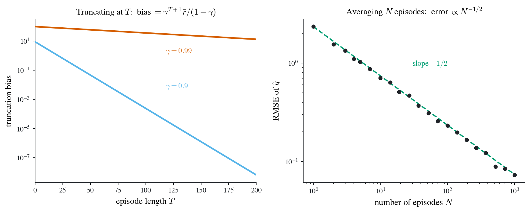
Figure 2.1: The two errors of Equation 2.7 die at different rates. Left: truncating each episode at \(T\) leaves a deterministic bias \(\gamma^{T+1}\bar{r}/(1-\gamma)\), geometric in \(T\) but with a rate set by \(\gamma\): at \(\gamma=0.9\) two hundred steps buys eight digits, at \(\gamma=0.99\) it buys barely one. Right: averaging \(N\) episodes leaves sampling error of order \(N^{-1/2}\) (dots simulated at \(\gamma=0.9\), \(T=200\); dashed line the \(-1/2\) reference slope), independent of \(\gamma\). Buying a digit of accuracy costs a fixed number of extra steps but a hundredfold increase in episodes.
The MC Basic algorithm
Substituting Equation 2.7 for the evaluation step of Equation 2.3 gives the simplest model-free algorithm there is.
NoteAlgorithm: MC Basic
Given an initial policy \(\pi_{0}\), at iteration \(k\), for every state \(s\in\mathcal{S}\) and every action \(a\in\mathcal{A}(s)\):
Collect sufficiently many episodes starting from \((s,a)\) and following \(\pi_{k}\).
Policy evaluation. Estimate the action value by the average return over those episodes: \[
q_{\pi_{k}}(s,a)\approx q_{k}(s,a)=\text{average return of all collected episodes}.
\]
Policy improvement. Act greedily with respect to the estimate: \[
a_{k}^{*}(s)=\argmax_{a}q_{k}(s,a),
\qquad
\pi_{k+1}(a\given s)=
\begin{cases}
1 & \text{if } a=a_{k}^{*}(s),\\
0 & \text{otherwise.}
\end{cases}
\]
MC Basic is policy iteration with one component swapped out:
Table 2.2: MC Basic is Howard policy iteration with sample averages in place of the exact evaluation step.
\(\argmax_{\pi}\{\mathbf{r}_{\pi}+\gamma\mathbf{P}_{\pi}\mathbf{v}_{\pi_{k}}\}\), reads the model
\(\argmax_{a}q_{k}(s,a)\), reads only the estimates
Needs the model
yes
no
Three remarks are worth making.
Why action values rather than state values. Because a state value cannot be turned into a decision on its own: converting \(v\) into a policy requires the model, as the improvement row of Table 2.2 shows. When the model is unavailable, estimate the object that is directly comparable across actions.
Exploration is smuggled in as an assumption. Step 1 assumes episodes can be started from any pair \((s,a)\), an assumption usually called exploring starts. It is doing all the work of exploration, and it is the one assumption we can actually get rid of, which the next section does.
Convergence. Policy iteration converges, and MC Basic is policy iteration, so MC Basic converges too, given sufficiently many episodes at every step.
Important
MC Basic is not a practical algorithm. It re-collects a fresh batch of episodes for every state-action pair at every iteration and throws away everything it learned from the previous batch, which makes it hopelessly sample-inefficient. Its purpose here is to isolate the one conceptual move (expectation \(\to\) sample average) before the efficiency questions arrive.
Exploring starts is an assumption about the environment, and usually a false one: you rarely get to reset a system into an arbitrary state-action pair. But notice what it was for. Greedy improvement in step 3 of MC Basic produces a policy that puts probability 1 on one action, so following it never generates data about the others, and an action never tried can never be found to be good. Exploring starts patched that from outside. The alternative is to patch it from inside, by refusing to make the policy fully greedy.
Definition 2.2 (ε-greedy policy) For \(\eps\in[0,1]\), the \(\eps\)-greedy policy with respect to \(q\) is \[
\pi(a\given s)=
\begin{cases}
1-\dfrac{\eps}{|\mathcal{A}(s)|}\big(|\mathcal{A}(s)|-1\big) & \text{if } a=\argmax_{a'}q(s,a'),\\[8pt]
\dfrac{\eps}{|\mathcal{A}(s)|} & \text{otherwise.}
\end{cases}
\]
Tip
Read Definition 2.2 as: with probability \(1-\eps\) act greedily, and with probability \(\eps\) pick uniformly at random among all actions. The greedy action keeps the largest share for any \(\eps<1\), so the policy still improves; but every action keeps probability at least \(\eps/|\mathcal{A}(s)|>0\), so no action is ever starved of data. Setting \(\eps=0\) recovers the greedy policy of MC Basic; setting \(\eps=1\) gives the uniform policy.
This is the exploitation-exploration trade-off, and \(\eps\) is the dial. An \(\eps\)-greedy policy is soft: every action has positive probability everywhere, so a single sufficiently long episode visits every \((s,a)\) pair infinitely often, provided every state is reachable under \(\pi\) from the start distribution and the induced chain is therefore irreducible on \(\mathcal{S}\). Exploring starts becomes unnecessary, because exploration is now a property of the policy rather than a favour asked of the environment.
Warning
Nothing is free. Restricting improvement to \(\eps\)-greedy policies means the algorithm converges to the best policy among \(\eps\)-greedy policies, not to the optimal policy, and the gap grows with \(\eps\). The standard fix is to shrink \(\eps\) toward zero as learning proceeds: explore aggressively while the estimates are bad, and act greedily once they are good.
2.3 Stochastic approximation
There are two reasons to leave RL for a section and study stochastic approximation on its own terms.
It is the essential preliminary for temporal-difference learning, and so the bridge from Monte Carlo RL to TD, the update Chapter 1 introduced as Equation 1.3 without justifying it.
It has many applications in economics beyond RL.
Motivating example: mean estimation
Return to the plainest possible version of the problem. Given a random variable \(X\) and iid samples \(\{x_{i}\}_{i=1}^{N}\), estimate \(\E[X]\) by
Because in RL almost everything is an expectation. Action values are expectations, Equation 2.6. Policy gradients are expectations. Every algorithm in this book is, underneath, a way of estimating a mean under awkward conditions.
The interesting question is not what\(\bar{x}\) is but how to compute it.
Batch. Collect all samples, then average. The drawback: if samples arrive one at a time over a period, nothing can be reported until the last one lands.
Incremental. Update the estimate as each sample arrives.
Let \(w_{k+1}\) denote the average of the first \(k\) samples,
Equation 2.8 is Equation 1.1 from Chapter 1 with the index shifted: here \(w_{k+1}\) is the mean of the first \(k\) samples, there \(\bar{x}_{k}\) is. The recursion is the same; only the label on the counter moved. This chapter uses the \(w\) convention because it is the one the stochastic-approximation literature writes the Robbins-Monro algorithm in.
Now generalize by replacing the step \(\tfrac{1}{k}\) with an arbitrary positive \(\alpha_{k}\):
NoteImplementation: the generalized incremental mean
The loop body is Equation 2.9 verbatim; alpha is either a float, giving a constant step, or an array of per-iteration steps \(\alpha_{k}\). Passing \(\alpha_{k}=1/k\) recovers the running mean of the first \(k\) samples exactly, whatever the starting guess \(w_{0}\), and that is what the closing assertion checks.
def mean_estimation_path(x, alpha, w0):"""Run w_{k+1} = w_k - alpha_k (w_k - x_k) over the sample stream x. Returns the path [w_1, ..., w_{N+1}] of estimates. """ n =len(x) a = np.full(n, alpha, float) if np.isscalar(alpha) else np.asarray(alpha, float) w = np.empty(n +1) w[0] = w0for k inrange(n): w[k +1] = w[k] - a[k] * (w[k] - x[k])return wx = np.random.default_rng(20260725).normal(0.0, 1.0, 50)w = mean_estimation_path(x, 1.0/ np.arange(1, 51), w0=99.0)assert np.allclose(w[1:], np.cumsum(x) / np.arange(1, 51)) # 1/k IS the running mean
This still converges to \(\E[X]\) under mild conditions on \(\{\alpha_{k}\}\). Those conditions are the subject of the rest of this section: Equation 2.9 is a special case of the Robbins-Monro algorithm.
The Robbins-Monro algorithm
Stochastic approximation (SA) refers to a broad class of stochastic iterative algorithms for root-finding or optimization. What makes it powerful, relative to gradient-based methods, is that it requires knowing neither the expression of the objective function nor its derivative. The Robbins-Monro (RM) algorithm is the pioneering work in the field; stochastic gradient descent is a special case of it, and it is what explains why Equation 2.9 works.
NotePreliminary: the gradient
For a scalar function \(J(w)\) with \(w=(w_{1},\dots,w_{m})\in\R^{m}\), the gradient is the column vector \[
\nabla_{w}J(w)=
\begin{bmatrix}
\partial J(w)/\partial w_{1}\\
\partial J(w)/\partial w_{2}\\
\vdots\\
\partial J(w)/\partial w_{m}
\end{bmatrix}.
\]
Problem statement. Find the root of
\[
g(w)=0,
\]
where \(w\in\R\) is the variable to be solved for and \(g:\R\to\R\).
NoteOn dimension
The theorem and proof below are stated for scalar\(w\), because the proof’s mean value theorem step needs a single intermediate point and that is a one-dimensional fact. Everything survives in \(\R^{m}\) with two substitutions: replace the mean value theorem by the integral form \(g(w_{k})-g(w^{*})=\big[\int_{0}^{1}\nabla_{w}g\big(w^{*}+\tau\Delta_{k}\big)\,d\tau\big]\Delta_{k}\), and replace condition 1 by a uniform spectral bound \(0<c_{1}I\preceq\nabla_{w}g(w)\preceq c_{2}I\) on the Jacobian. The vector case is what Chapters 3 and 4 actually use, since there \(w\) and \(\theta\) are parameter vectors.
Tip
Root-finding is less special than it looks. If \(J(w)\) is an objective to be minimized, its first-order condition \(g(w)=\nabla_{w}J(w)=0\) is a root-finding problem. Optimization is root-finding on the gradient.
How to solve \(g(w)=0\) splits along the same line as everything else in this chapter:
Model-based. If the expression of \(g\) is known, standard numerical algorithms apply.
Model-free. What if the expression of \(g\) is unknown, and all we obtain are noisy observations of its values?
where \(w_{k}\) is the \(k\)-th estimate of the root, \(\tilde{g}(w_{k},\eta_{k})=g(w_{k})+\eta_{k}\) is the \(k\)-th noisy observation, and \(\alpha_{k}>0\) is the step size.
Theorem 2.1 (Robbins-Monro) In the RM algorithm Equation 2.10, suppose
\(0<c_{1}\leq\nabla_{w}g(w)\leq c_{2}\) for all \(w\);
\(\sum_{k=1}^{\infty}\alpha_{k}=\infty\) and \(\sum_{k=1}^{\infty}\alpha_{k}^{2}<\infty\);
\(\E[\eta_{k}\given\mathcal{H}_{k}]=0\) and \(\E[\eta_{k}^{2}\given\mathcal{H}_{k}]\leq C\) almost surely, for a constant \(C\) not depending on \(k\),
where \(\mathcal{H}_{k}=\{w_{k},w_{k-1},\dots\}\). Then \(w_{k}\) converges with probability 1 to the root \(w^{*}\) satisfying \(g(w^{*})=0\).
TipReading the three conditions
Each condition rules out one way the iteration could fail.
\(g\) is increasing and well-conditioned. The lower bound \(c_{1}>0\) makes the root unique and guarantees the update always points toward it; the upper bound \(c_{2}\) stops the steps from overshooting arbitrarily far.
The steps are large enough in total, small enough individually.\(\sum\alpha_{k}=\infty\) means the iteration can still travel an unbounded distance and so cannot stall short of the root no matter where it starts. \(\sum\alpha_{k}^{2}<\infty\) means \(\alpha_{k}\to0\) fast enough that the accumulated noise stays finite and the estimate settles. The canonical choice \(\alpha_{k}=1/k\) satisfies both, which is exactly the step in Equation 2.8.
The noise is zero-mean with finite variance. Unbiased observations, so errors cancel rather than accumulate into a drift.
This is the theorem Chapter 1 gestured at when it noted that a constant\(\alpha\) violates condition 2: \(\sum\alpha=\infty\) holds but \(\sum\alpha^{2}=\infty\) too, so the estimate never settles and instead fluctuates around the truth. That is a price paid deliberately, in exchange for the ability to track a moving target.
Why the Robbins-Monro theorem is true
Theorem 2.1 is usually quoted and not proved. It is worth proving, because the argument is short once the right tool is in hand, and because that same tool proves every convergence result in the next chapter.
The tool is a classical result of Dvoretzky on stochastic processes of a particular shape.
Theorem 2.2 (Dvoretzky) Consider the stochastic process \[
\Delta_{k+1}=(1-\alpha_{k})\Delta_{k}+\beta_{k}\eta_{k},
\tag{2.11}\] where \(\{\alpha_{k}\},\{\beta_{k}\},\{\eta_{k}\}\) are stochastic sequences with \(\alpha_{k}\geq0\) and \(\beta_{k}\geq0\). Then \(\Delta_{k}\) converges to zero almost surely if
\(\sum_{k}\alpha_{k}=\infty\), \(\sum_{k}\alpha_{k}^{2}<\infty\), and \(\sum_{k}\beta_{k}^{2}<\infty\) uniformly almost surely;
\(\E[\eta_{k}\given\mathcal{H}_{k}]=0\) and \(\E[\eta_{k}^{2}\given\mathcal{H}_{k}]\leq C\) almost surely,
where \(\mathcal{H}_{k}=\{\Delta_{k},\Delta_{k-1},\dots,\eta_{k-1},\dots,\alpha_{k-1},\dots,\beta_{k-1},\dots\}\) is the history.
Tip
Read Equation 2.11 as a tug of war. The factor \((1-\alpha_{k})\) contracts the error toward zero; the term \(\beta_{k}\eta_{k}\) kicks it away at random. Condition 1 says the contraction wins: \(\sum\alpha_{k}=\infty\) makes the pulling relentless, while \(\sum\alpha_{k}^{2},\sum\beta_{k}^{2}<\infty\) make the accumulated kicking finite. Condition 2 says the kicks are unbiased with bounded variance, so they cancel rather than drift.
Two things separate Theorem 2.2 from the naive argument. First, \(\alpha_{k}\) and \(\beta_{k}\) are allowed to be random, and to depend on the history: that is exactly what is needed below, where the effective step size turns out to depend on the current iterate. Second, the conclusion is almost-sure convergence, not convergence in mean. The proof of Theorem 2.2 itself rests on convergence results for quasimartingales and is not reproduced here; the RM theorem is a corollary of it, and that corollary is the part worth seeing.
NoteProof of the Robbins-Monro theorem
Let \(w^{*}\) be the root, so \(g(w^{*})=0\), and write the RM algorithm Equation 2.10 with the noisy observation expanded: \[
w_{k+1}=w_{k}-\alpha_{k}\tilde{g}(w_{k},\eta_{k})=w_{k}-\alpha_{k}\big[g(w_{k})+\eta_{k}\big].
\] Subtract \(w^{*}\) from both sides and insert \(g(w^{*})=0\) for free: \[
w_{k+1}-w^{*}=w_{k}-w^{*}-\alpha_{k}\big[g(w_{k})-g(w^{*})+\eta_{k}\big].
\] By the mean value theorem there is a \(w_{k}'\) between \(w_{k}\) and \(w^{*}\) with \[
g(w_{k})-g(w^{*})=\nabla_{w}g(w_{k}')\,(w_{k}-w^{*}).
\] Writing \(\Delta_{k}\defeq w_{k}-w^{*}\) for the error and substituting, \[
\begin{aligned}
\Delta_{k+1}&=\Delta_{k}-\alpha_{k}\big[\nabla_{w}g(w_{k}')\Delta_{k}+\eta_{k}\big]\\
&=\Big[1-\underbrace{\alpha_{k}\nabla_{w}g(w_{k}')}_{\defeq\,\bar{\alpha}_{k}}\Big]\Delta_{k}+\underbrace{\alpha_{k}}_{\beta_{k}}(-\eta_{k}),
\end{aligned}
\] which is precisely Equation 2.11. It remains to check its two conditions.
Condition 1. By hypothesis 1 of Theorem 2.1, \(0<c_{1}\leq\nabla_{w}g(w)\leq c_{2}\) for every \(w\), so the effective step is sandwiched: \[
c_{1}\alpha_{k}\leq\bar{\alpha}_{k}\leq c_{2}\alpha_{k}.
\] Hypothesis 2 gives \(\sum_{k}\alpha_{k}=\infty\) and \(\sum_{k}\alpha_{k}^{2}<\infty\); the sandwich transfers both to \(\bar{\alpha}_{k}\), since \(\sum\bar{\alpha}_{k}\geq c_{1}\sum\alpha_{k}=\infty\) and \(\sum\bar{\alpha}_{k}^{2}\leq c_{2}^{2}\sum\alpha_{k}^{2}<\infty\). And \(\sum_{k}\beta_{k}^{2}=\sum_{k}\alpha_{k}^{2}<\infty\).
Condition 2. Hypothesis 3 gives \(\E[\eta_{k}\given\mathcal{H}_{k}]=0\) and the uniform bound \(\E[\eta_{k}^{2}\given\mathcal{H}_{k}]\leq C\), which is what Theorem 2.2 asks for; pointwise finiteness at each \(k\) would not be enough, since the constant must not drift with \(k\). Negating \(\eta_{k}\) changes neither.
Both conditions hold, so Theorem 2.2 gives \(\Delta_{k}\to0\) almost surely, that is \(w_{k}\to w^{*}\). \(\square\)
Note
Notice where hypothesis 1 of Theorem 2.1 was spent. The lower bound \(c_{1}>0\) keeps \(\sum\bar{\alpha}_{k}=\infty\) from collapsing, which is what stops the iteration stalling at a point where \(g\) has gone flat; the upper bound \(c_{2}\) keeps \(\sum\bar{\alpha}_{k}^{2}\) finite, which is what stops a steep \(g\) from turning a small step into a large jump. The condition is not a technicality but the precise statement that \(g\) is neither too flat nor too steep anywhere.
Notice also that \(\bar{\alpha}_{k}\) depends on \(w_{k}'\), hence on the iterate, hence on the history. A version of Theorem 2.2 requiring deterministic step sizes would not close this argument.
Write mean estimation as root-finding. Define \[
g(w)=w-\E[X],
\] whose root is \(w^{*}=\E[X]\). Note we do not know the expression of \(g\): it contains the very quantity we are trying to estimate.
Identify the noisy observation. With a sample \(x\) in hand we can evaluate \[
\tilde{g}(w,x)=w-x,
\] which is exactly \(g\) plus zero-mean noise: \[
\begin{aligned}
\tilde{g}(w,x)&=w-x\\
&=w-x+\E[X]-\E[X]\\
&=\underbrace{\big(w-\E[X]\big)}_{g(w)}+\underbrace{\big(\E[X]-x\big)}_{\eta}.
\end{aligned}
\]
Apply RM. Substituting into Equation 2.10, \[
w_{k+1}=w_{k}-\alpha_{k}\,\tilde{g}(w_{k},x_{k})=w_{k}-\alpha_{k}(w_{k}-x_{k}),
\] which is precisely Equation 2.9. Its convergence is therefore not a separate fact to be proved but a corollary of Theorem 2.1.
Note
Check the hypotheses hold here: \(\nabla_{w}g(w)=1\), so condition 1 is satisfied with \(c_{1}=c_{2}=1\); and \(\eta=\E[X]-x\) has mean zero by construction, so condition 3 holds whenever \(X\) has finite variance. Only condition 2 constrains the algorithm, and it is a constraint on the step sizes we choose, not on the problem.
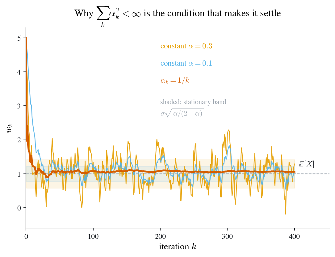
Since condition 2 is the only one with any bite here, it is worth seeing what it does.
One sample stream, three step-size rules, run through @eq-mean-general
fig, ax = new_ax(6.6, 4.4)mu, sigma, n =1.0, 1.0, 400x = RNG.normal(mu, sigma, n) # one shared sample streamk = np.arange(1, n +1)ax.axhline(mu, color=GREY, lw=0.9, ls="--", zorder=2)for alpha, colour in ((0.30, COL["orange"]), (0.10, COL["sky"])): w = mean_estimation_path(x, alpha, w0=5.0) ax.plot(np.arange(n +1), w, color=colour, lw=1.0, alpha=0.9, zorder=3)# stationary std of the constant-step recursion: sigma * sqrt(a/(2-a)) band = sigma * np.sqrt(alpha / (2- alpha)) ax.fill_between([0, n], mu - band, mu + band, color=colour, alpha=0.10, zorder=1)w = mean_estimation_path(x, 1.0/ k, w0=5.0)ax.plot(np.arange(n +1), w, color=COL["vermilion"], lw=2.2, zorder=5)ax.set_xlim(0, n *1.13) # headroom on the right for the E[X] tagax.set_ylim(-0.6, 5.3)ax.set_xlabel(r"iteration $k$")ax.set_ylabel(r"$w_k$")# Direct labels live in the empty upper-right quadrant, clear of the paths.label_at(ax, n *1.015, mu +0.28, r"$\mathbb{E}[X]$", color=INK, fontsize=9.5)label_at(ax, n *0.50, 4.75, r"constant $\alpha=0.3$", color=COL["orange"], fontsize=9.5)label_at(ax, n *0.50, 4.25, r"constant $\alpha=0.1$", color=COL["sky"], fontsize=9.5)label_at(ax, n *0.50, 3.75, r"$\alpha_k=1/k$", color=COL["vermilion"], fontsize=9.5)label_at( ax, n *0.50,3.20,"shaded: stationary band\n"r"$\sigma\sqrt{\alpha/(2-\alpha)}$", color=GREY, fontsize=8.5, va="top",)ax.set_title(r"Why $\sum_k \alpha_k^2 < \infty$ is the condition that makes it settle")plt.show()
Figure 2.2: The recursion Equation 2.9 run on one shared stream of draws \(x_{k}\sim N(1,1)\) from the same starting point \(w_{1}=5\), under three step-size rules. With \(\alpha_{k}=1/k\) (thick) both parts of condition 2 hold and the path settles onto \(\E[X]\). With a constant\(\alpha\), \(\sum_{k}\alpha_{k}^{2}=\infty\), so the path never settles: it keeps fluctuating inside a band of width \(\sigma\sqrt{\alpha/(2-\alpha)}\) (shaded), wider for larger \(\alpha\). The bargain of a constant step, exactly as described in Chapter 1: the estimate gives up convergence to a point in exchange for never going deaf.
Stochastic gradient descent
The same argument, applied to a gradient instead of to a residual, produces the workhorse of everything that follows. Suppose we want to minimize
\[
J(w)=\E\big[f(w,X)\big]
\tag{2.12}\]
over \(w\), where the expectation is over a random variable \(X\) we can sample but whose distribution we do not know. There are three ways to descend.
Table 2.3: Three ways down the same objective Equation 2.12. Only the last is usable when samples arrive one at a time and the distribution is unknown.
It replaces the true gradient by a single-sample estimate of it, which is a wildly noisy substitute. That it works at all is Theorem 2.1.
NoteDerivation: SGD is Robbins-Monro on the first-order condition
Minimizing Equation 2.12 means solving its first-order condition, which is a root-finding problem in the sense of the previous section: \[
g(w)\defeq\nabla_{w}J(w)=\E\big[\nabla_{w}f(w,X)\big]=0 ,
\] where the interchange of \(\nabla_{w}\) and \(\E\) assumes \(f(\cdot,x)\) is differentiable and that \(\|\nabla_{w}f(w,X)\|\) is dominated near \(w\) by an integrable envelope, so dominated convergence applies to the difference quotients. We cannot evaluate \(g\), since it is an expectation over an unknown distribution. But with a sample \(x\) in hand we can evaluate \(\nabla_{w}f(w,x)\), and it is \(g\) plus zero-mean noise: \[
\tilde{g}(w,x)=\nabla_{w}f(w,x)
=\underbrace{\E\big[\nabla_{w}f(w,X)\big]}_{g(w)}
+\underbrace{\Big(\nabla_{w}f(w,x)-\E\big[\nabla_{w}f(w,X)\big]\Big)}_{\eta} .
\] Substituting into the RM algorithm Equation 2.10 gives exactly Equation 2.13. So SGD is not a separate algorithm with its own theory: it is RM applied to a gradient, and its convergence conditions are the three of Theorem 2.1, read on \(g=\nabla_{w}J\).
The circle closes on the example this section started from.
Example 2.1 (Mean estimation is SGD) Take \(f(w,x)=\tfrac{1}{2}|w-x|^{2}\), so that \(J(w)=\tfrac{1}{2}\E|w-X|^{2}\) is minimized at \(w^{*}=\E[X]\). Then \(\nabla_{w}f(w,x)=w-x\), and Equation 2.13 reads \[
w_{k+1}=w_{k}-\alpha_{k}(w_{k}-x_{k}),
\] which is Equation 2.9 once more. Mean estimation is a special case of SGD, which is a special case of Robbins-Monro. All three are the same recursion seen at three levels of generality.
Important
Equation 2.13 is the engine of the rest of the book. Chapter 3 uses it to fit a parametric value function \(\hat{v}(s,w)\) by descending the squared error, which is what turns tabular TD learning into TD learning with function approximation. Chapter 4 runs it in the other direction, as stochastic gradient ascent on the value of a parameterized policy, which is what policy gradient methods are.