1  The Basic Idea of RL, and Its Link to Dynamic Programming

\[ \newcommand{\E}{\mathbb{E}} \newcommand{\R}{\mathbb{R}} \newcommand{\Prob}{\mathbb{P}} \newcommand{\BR}{\operatorname{BR}} \newcommand{\eps}{\varepsilon} \newcommand{\given}{\,\vert\,} \newcommand{\argmax}{\operatorname*{arg\,max}} \newcommand{\argmin}{\operatorname*{arg\,min}} \newcommand{\sm}{\setminus} \newcommand{\defeq}{\equiv} \]

This first chapter follows Ben Moll’s Lecture 1. The one idea to keep in mind throughout: reinforcement learning is Monte-Carlo dynamic programming. It uses the same Bellman recursions, but with expectations estimated from samples instead of computed from a known model.

NoteSource:

Ben Moll’s RL lecture slides, Lecture 1.

1.1 The basic idea of RL

For a random variable \(x\), how can we compute \(\E[x]\)? There are two approaches.

  1. Exact. If we know the distribution \(p(x)\), integrate: \[ \E[x]=\int x\,p(x)\,dx . \]
  2. Monte Carlo. If we do not know \(p(x)\) but can sample \(\vec{x}=[x_{1},\dots,x_{N}]'\), average: \[ \E[x]\approx \bar{x}=\frac{1}{N}\sum_{i=1}^{N}x_{i} . \]

The Monte-Carlo mean can be built up incrementally. Writing \(\bar{x}_{k}=\tfrac{1}{k}\sum_{i=1}^{k}x_{i}\) for the running mean of the first \(k\) samples, a one-line rearrangement gives the recursion

\[ \bar{x}_{k}=\bar{x}_{k-1}+\frac{1}{k}\,(x_{k}-\bar{x}_{k-1}). \tag{1.1}\]

Tip

Read Equation 1.1 as old estimate \(+\) step \(\times\) (new sample \(-\) old estimate). The step size \(\tfrac{1}{k}\) is the learning rate. Replacing it with a constant \(\alpha\) is precisely what turns averaging into learning, the recurring theme of everything below.

Computing a value function

Definition 1.1 (Markov reward process) A Markov reward process (MRP) assigns to each starting state \(s_{0}\) the discounted expected reward \[ v(s_{0})=\E\!\left[\sum_{t=0}^{\infty}\beta^{t}r(s_{t})\right], \] where the state \(s_{t}\) follows an exogenous Markov process and \(\beta\in(0,1)\) is the discount factor.

As before, there are two ways to obtain \(v\).

  1. Dynamic programming. If we know the transition density \(p(s'\given s)\), then \(v\) solves the fixed point \[ v(s)=r(s)+\beta\int v(s')\,p(s'\given s)\,ds' . \tag{1.2}\]
  2. Monte Carlo. If we cannot evaluate \(p\) but can sample trajectories \(\{s_{t}^{i}\}_{t=0}^{T}\), average the realized returns: \[ v(s_{0})\approx \hat{v}(s_{0})=\frac{1}{N}\sum_{i=1}^{N}\sum_{t=0}^{T}\beta^{t}r(s_{t}^{i}). \]

Averaging whole trajectories is wasteful: it waits for a trajectory to finish before updating. Instead we can update \(\hat{v}\) at every step \(t\) of every trajectory \(k\), using the incremental rule Equation 1.1 with a constant learning rate \(\alpha\):

\[ \hat{v}_{t+1}^{k}(s_{t}^{k})=\hat{v}_{t}^{k}(s_{t}^{k})+\alpha\big[\,r(s_{t}^{k})+\beta\,\hat{v}_{t}^{k}(s_{t+1}^{k})-\hat{v}_{t}^{k}(s_{t}^{k})\,\big]. \tag{1.3}\]

This is the TD(0) update. Where does it come from?

Start from the dynamic-programming fixed point Equation 1.2 and read it as an expectation: \[ v(s)=r(s)+\beta\int v(s')\,p(s'\given s)\,ds' =\E_{s'\sim p(\cdot\given s)}\big[\,\underbrace{r(s)+\beta v(s')}_{Y\,\defeq\,r(s)+\beta v(s')}\,\big]. \] So computing \(v(s)\) is computing \(\E[Y]\), and we already know how to estimate an expectation incrementally via Equation 1.1, with the learning rate relaxed to a constant \(\alpha\).

At trajectory \(k\) the realized value of \(Y\) is \(r(s^{k})+\beta v(s'^{k})\). The catch: we do not have the true \(v(s'^{k})\). So we bootstrap: plug in the current estimate \(\hat{v}^{k}\) in its place: \[ x_{k}=r(s^{k})+\beta\,\hat{v}^{k}(s'^{k}). \] If \(\hat{v}^{k}\to v\) then \(x_{k}\to Y\), so the target is asymptotically unbiased. Feeding \(x_{k}\) into the incremental rule \(\bar{x}_{k}=\bar{x}_{k-1}+\alpha(x_{k}-\bar{x}_{k-1})\), with \(\bar{x}_{k}=\hat{v}'^{k}(s^{k})\) the updated estimate and \(\bar{x}_{k-1}=\hat{v}^{k}(s^{k})\) the old one (a prime marks the post-update value), gives \[ \begin{aligned} \hat{v}'^{k}(s^{k}) &=\hat{v}^{k}(s^{k})+\alpha\big[\,r(s^{k})+\beta\,\hat{v}^{k}(s'^{k})-\hat{v}^{k}(s^{k})\,\big] \\ &=(1-\alpha)\,\hat{v}^{k}(s^{k})+\alpha\big[\,r(s^{k})+\beta\,\hat{v}^{k}(s'^{k})\,\big], \end{aligned} \] which is Equation 1.3 written one step at a time.

Tip

The last line says the new estimate is a convex combination of the old estimate and the bootstrapped target, with weights \((1-\alpha,\,\alpha)\). The bracketed quantity \(r+\beta\hat{v}(s')-\hat{v}(s)\) is the temporal-difference error: the gap between the one-step-ahead target and the current guess.

NoteWhy a constant step size?

The average in Equation 1.1 uses a shrinking step \(\tfrac{1}{k}\) because it estimates the mean of a fixed distribution: every sample deserves equal weight, and the estimate converges (its variance falls like \(1/k\)).

The TD target \(r+\beta\,\hat{v}(s')\) is different: it is non-stationary. It moves as \(\hat{v}\) is updated (that is exactly what bootstrapping does), and as the policy changes. A step that decays to zero would freeze the early, low-quality estimates in place and never catch up to the moving target.

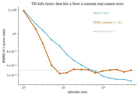
A constant \(\alpha\) instead keeps a fixed weight on recent samples (an exponentially recency-weighted average, \(\hat{v}\leftarrow(1-\alpha)\hat{v}+\alpha\cdot(\text{target})\)), so the estimate keeps chasing the target. The price: it no longer converges to a point but fluctuates around the truth, with a stationary standard deviation \(\propto\sqrt{\alpha}\) (it violates the Robbins-Monro conditions \(\sum_{t}\alpha_{t}=\infty,\ \sum_{t}\alpha_{t}^{2}<\infty\)). Genuine convergence needs \(\alpha\) to decay over time. So a constant step trades asymptotic precision for the ability to track.

The trajectory average and the TD(0) update estimate the same \(v\), but they trade off very differently:

Table 1.1: Monte Carlo vs. TD(0) as estimators of the value function.
Trajectory average (MC) TD(0) (bootstrap)
Target realized return \(\sum_{t}\beta^{t}r\) \(r+\beta\,\hat{v}(s')\)
Bias unbiased biased for finite \(\hat{v}\) (unbiased only as \(\hat{v}\to v\))
Variance high (sums many random steps) low (one random step plus a bootstrap)
Updates only once the trajectory ends every step, online

TD buys much lower variance at the cost of a little bias, and trades “wait until the end” for “update online.” The two are endpoints of a spectrum: \(n\)-step returns and TD(\(\lambda\)) interpolate between them.

Figure 1.1: The trade in Table 1.1, measured. Both estimators are shown the same episodes from a five-state discounted Markov reward process, and scored by the error of \(\hat{v}\) across all states. TD(0) falls faster at small budgets, because one random step carries far less variance than a whole trajectory. But a constant step size never settles: TD flattens onto a noise floor whose height is set by \(\alpha\), while Monte Carlo, which keeps averaging, eventually crosses below it. Which estimator is better is therefore a question about the sample budget, not a fact about the estimators.

Reinforcement learning and deep learning

Often we approximate the value function by a parametric family \[ \hat{V}(s,w), \] where \(w\) is a parameter vector, for instance the weights of a neural network. RL with a neural-network approximator is what people call deep reinforcement learning.

Note

RL and deep learning are orthogonal. RL is about how to estimate values and policies from sampled experience; the network is merely one choice of function approximator. Either can be swapped out without the other.