5 Dynamic Games with Incomplete Information
\[ \newcommand{\E}{\mathbb{E}} \newcommand{\R}{\mathbb{R}} \newcommand{\Prob}{\mathbb{P}} \newcommand{\BR}{\operatorname{BR}} \newcommand{\eps}{\varepsilon} \newcommand{\given}{\,\vert\,} \newcommand{\argmax}{\operatorname*{arg\,max}} \newcommand{\argmin}{\operatorname*{arg\,min}} \newcommand{\sm}{\setminus} \newcommand{\defeq}{\equiv} \]
This chapter brings together the two threads of the previous two chapters: the sequential structure of Chapter 3 and the private information of Chapter 4. When players move in turn but some of them do not know others’ types, the difficulty is that subgame-perfect equilibrium often has nothing to say — too few proper subgames exist for backward induction to bite. The remedy is perfect Bayesian equilibrium, which equips each player with a belief about where they are in the tree and demands that strategies be optimal given those beliefs. We develop the concept on a chain-store example, apply it to signaling games (Spence’s model of education as a costly signal), sharpen it with the Cho–Kreps intuitive criterion, and finally study cheap talk, where the signal is costless and the question becomes how much information can be credibly transmitted at all.
5.1 A motivating example
The chain-store game with complete information
A potential entrant (player 1) decides whether to stay out (\(S\)) or enter (\(E\)) a market served by an incumbent (player 2). If the entrant stays out, the incumbent keeps the market and payoffs are \((0,2)\). If the entrant enters, the incumbent chooses to fight (\(F\)) — a price war that hurts both, paying \((-1,-1)\) — or to accommodate (\(A\)), paying \((1,1)\). The tree is shown in Figure 5.1.
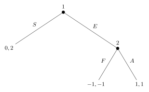
This game has two pure-strategy Nash equilibria, \((S,F)\) and \((E,A)\), but only \((E,A)\) is subgame perfect (Definition 3.11). The profile \((S,F)\) rests on a non-credible threat: the incumbent promises to fight, which keeps the entrant out, but if entry actually occurred the incumbent would prefer to accommodate (\(1 > -1\)). Subgame perfection requires sequential rationality both on and off the equilibrium path, and so eliminates \((S,F)\); Nash equilibrium does not.
The chain-store game with incomplete information
Now suppose the entrant has private information about its own strength. Nature first draws the entrant’s type: competent (\(C\)) with probability \(p\), or weak (\(W\)) with probability \(1-p\). The competent entrant’s payoffs are as before; the weak entrant’s are worse — fighting it yields the incumbent \(0\) rather than \(-1\), and the weak entrant earns \(-2\) if fought and \(-1\) if accommodated. Crucially, only the entrant knows its own type: the incumbent, who moves after observing entry, cannot tell a competent entrant from a weak one. The extensive form is Figure 5.2.
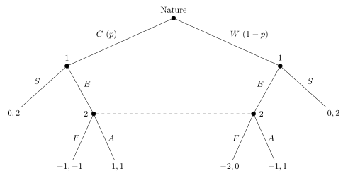
Because the entrant now has two information sets — one per type — a pure strategy specifies an action for each, so \[ S_1 = \{SS,\ SE,\ ES,\ EE\}, \] where the first letter is the action of the competent type and the second that of the weak type (e.g. \(ES\) = competent enters, weak stays out). The incumbent still has a single information set and acts \(S_2 = \{F, A\}\). Computing the expected payoffs over Nature’s draw gives the normal form in Table 5.1.
| \(F\) | \(A\) | |
|---|---|---|
| \(SS\) | \(0,\ 2\) | \(0,\ 2\) |
| \(SE\) | \(-2(1-p),\ 2p\) | \(-(1-p),\ 2p+(1-p)\) |
| \(ES\) | \(-p,\ -p+2(1-p)\) | \(p,\ p+2(1-p)\) |
| \(EE\) | \(-p-2(1-p),\ -p\) | \(p-(1-p),\ p+(1-p)\) |
Specialise to \(p=\tfrac12\) for concreteness:
| \(F\) | \(A\) | |
|---|---|---|
| \(SS\) | \(0,\ 2\) | \(0,\ 2\) |
| \(SE\) | \(-1,\ 1\) | \(-\tfrac12,\ \tfrac32\) |
| \(ES\) | \(-\tfrac12,\ \tfrac12\) | \(\tfrac12,\ \tfrac32\) |
| \(EE\) | \(-\tfrac32,\ -\tfrac12\) | \(0,\ 1\) |
There are two pure-strategy Nash equilibria, \((SS,F)\) and \((ES,A)\). Since the extensive-form game can equally be cast as a Bayesian game, these are precisely its Bayesian Nash equilibria (Definition 4.3). Both are subgame perfect — yet \((SS,F)\) involves exactly the kind of non-credible behaviour we wanted to rule out: accommodating is better than fighting for the incumbent regardless of the entrant’s type (\(A\) weakly dominates \(F\) in the incumbent’s row of payoffs), so the threat to fight should not deter entry.
Why subgame perfection has no bite
The reason subgame perfection fails to eliminate \((SS,F)\) is structural. The only proper subgame of Figure 5.2 is the whole game: because the incumbent’s two nodes lie in a single information set, no smaller subtree begins at a single node. With only the trivial subgame, every Nash equilibrium is automatically subgame perfect — Nash \(=\) SPE.
This is a general feature of dynamic games with incomplete information: although the incumbent observes the entrant’s action, it does not observe the entrant’s type, so the information set spanning both types prevents the tree from splitting into proper subgames. Subgame perfection therefore has “no bite,” and we need a finer concept that extends sequential rationality to information sets inside a game. That concept is perfect Bayesian equilibrium.
5.2 Perfect Bayesian equilibrium
The idea is to attach to each information set a belief — a probability distribution over the nodes it contains — and to require each player to act optimally given that belief. We begin by distinguishing the information sets that the play actually reaches.
Definition 5.1 (On and off the equilibrium path) Let \(\sigma^* = (\sigma_1^*, \dots, \sigma_n^*)\) be a Bayesian Nash equilibrium profile of strategies in a game of incomplete information. An information set is on the equilibrium path if, given \(\sigma^*\) and the distribution of types, it is reached with positive probability; it is off the equilibrium path if, given \(\sigma^*\) and the distribution of types, it is reached with probability zero.
In the chain-store game, every information set is on the path under \((ES,A)\), whereas under \((SS,F)\) the incumbent’s information set is off the path — entry never occurs, so the incumbent is never called to move.
Definition 5.2 (System of beliefs) A system of beliefs \(\mu\) of an extensive-form game assigns a probability distribution over decision nodes to every information set. That is, for every information set \(h \in H\) and every decision node \(x \in h\), \(\mu(x) \in [0,1]\) is the probability that the player who moves at \(h\) assigns to being at \(x\), where \[ \sum_{x \in h} \mu(x) = 1 \qquad \text{for every } h \in H . \]
A perfect Bayesian equilibrium is then a strategy profile together with a system of beliefs satisfying four requirements. Because these are stated as informal “requirements” rather than as numbered results, we render them as bold-labelled prose rather than numbered definitions.
Requirement 1 (Beliefs exist). Every player has a well-defined belief over where they are in each of their information sets. That is, the game comes equipped with a system of beliefs \(\mu\).
Requirement 2 (Consistency). Let \(\sigma^* = (\sigma_1^*, \dots, \sigma_n^*)\) be a Bayesian Nash equilibrium profile. On the equilibrium path, beliefs must be consistent with Bayes’ rule. Given \(\sigma^*\) and Nature’s move, let \(\Prob^{\sigma^*}(x)\) be the probability that node \(x\) is reached, and \[ \Prob^{\sigma^*}(h) \equiv \sum_{x \in h} \Prob^{\sigma^*}(x). \] An information set \(h\) is on the path iff \(\Prob^{\sigma^*}(h) > 0\), and in that case Requirement 2 demands \[ \mu(x) = \frac{\Prob^{\sigma^*}(x)}{\Prob^{\sigma^*}(h)} \qquad \text{for all } x \in h . \tag{5.1}\]
Requirement 3 (Off-path beliefs). At information sets that are off the equilibrium path — where \(\Prob^{\sigma^*}(h) = 0\), so Bayes’ rule does not apply — any belief may be assigned. No restriction at all is imposed on off-path beliefs.
Requirement 4 (Sequential rationality). Given their beliefs, players’ strategies must be sequentially rational: at every information set a player plays a best response to their belief. If \(h\) is player \(i\)’s information set, then \(\sigma_i\) is sequentially rational at \(h\) given \(\sigma_{-i}\) and \(\mu\) if \[ \E\!\big[v_i(\sigma_i, \sigma_{-i}, \theta) \given h, \mu\big] \ge \E\!\big[v_i(s_i, \sigma_{-i}, \theta) \given h, \mu\big] \qquad \text{for all } s_i . \tag{5.2}\] In words: conditional on \(h\) being reached, playing \(\sigma_i\) is at least as good as any alternative given \(\sigma_{-i}\) and \(\mu\).
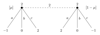
To see Requirement 4 in isolation, consider Figure 5.3, where a single player moves at an information set with two nodes (beliefs \(\mu\) and \(1-\mu\)) and three actions \(a, b, c\). The payoffs are \((-1,0,2)\) at the left node and \((2,0,-1)\) at the right. Whatever the belief, action \(b\) yields \(0\), while \(a\) yields \(-\mu + 2(1-\mu) = 2 - 3\mu\) and \(c\) yields \(2\mu - (1-\mu) = 3\mu - 1\); the larger of these two is at least \(\tfrac12 > 0\) for every \(\mu \in [0,1]\). So \(b\) is never a best response: it is not sequentially rational under any belief. (This is why, in the chain-store game, \((SS,F)\) is not sequentially rational for any belief about the entrant’s type — the incumbent always strictly prefers to accommodate.)
Definition 5.3 (Perfect Bayesian equilibrium) A Bayesian Nash equilibrium profile \(\sigma^* = (\sigma_1^*, \dots, \sigma_n^*)\) together with a system of beliefs \(\mu\) constitutes a perfect Bayesian equilibrium (PBE) of an \(n\)-player game if they satisfy Requirements 1–4.
A PBE thus packages rationality (best responses at every information set), correct beliefs on the path (Bayes’ rule), and unrestricted but fixed beliefs off the path. The freedom in off-path beliefs is the source of multiplicity we return to when discussing refinements. One case, however, is clean: when the candidate equilibrium reaches every information set, Bayes’ rule pins down the beliefs uniquely.
Proposition 5.1 (Uniqueness of consistent beliefs on the path) If a profile \(\sigma^* = (\sigma_1^*, \dots, \sigma_n^*)\) is a Bayesian Nash equilibrium of a Bayesian game \(\Gamma\), and if \(\sigma^*\) induces all information sets to be reached with positive probability, then \(\sigma^*\), together with the belief system \(\mu^*\) uniquely derived from \(\sigma^*\) and the distribution of types, constitutes a perfect Bayesian equilibrium of \(\Gamma\).
Proof. The handout states this without proof. The point is immediate from Requirement 2: if every information set is on the path, then \(\Prob^{\sigma^*}(h) > 0\) at each \(h\), so Equation 5.1 applies everywhere and determines \(\mu^*\) uniquely; no off-path freedom remains. Sequential rationality (Requirement 4) coincides with the best-response condition already guaranteed by the Bayesian Nash property. Hence there is exactly one consistent belief system and the BNE is automatically a PBE. \(\square\)
5.3 Signaling games
In a signaling game an informed player 1 (the sender) observes a private type drawn by Nature and chooses an action — a signal — that an uninformed player 2 (the receiver) observes before responding. The receiver cannot see the type, only the signal, so the sender’s action may convey information. The central question is when a signal is credible: when does the receiver rationally infer something about the type from the signal?
Many economic phenomena are signals in exactly this sense:
- a warranty signals that a manufacturer believes its product is reliable;
- retaining equity at IPO signals that an entrepreneur believes the firm is valuable;
- conspicuous consumption signals wealth;
- education signals ability.
The recurring logic, due to Michael Spence (Nobel Prize, 2001), is that a signal is credible precisely when it is differentially costly across types: the “good” type can afford the signal that the “bad” type would find too expensive to mimic.
5.4 Education signaling
We study Spence’s model in its sharpest form, where education is completely unproductive and yet still transmits information. Nature draws player 1’s skill: high (\(H\)) with probability \(p \in (0,1)\), or low (\(L\)) with probability \(1-p\), common knowledge. Player 1 (he) learns his type and chooses an MBA degree (\(D\)) or to stop at the undergraduate level (\(U\)). Education is costly, and the cost differs by type: \[ c_H = 2 < c_L = 5, \qquad \text{(no cost if } U). \] Player 2 (she, the employer) observes only whether player 1 holds the degree, then assigns him to be a manager (\(M\)) or a blue-collar worker (\(B\)), paying wage \(w_M = 10\) or \(w_B = 6\), with \(w_M > w_B\).
Education does not raise productivity. Net profit to the employer (output minus wage) depends only on intrinsic skill and the job:
| \(M\) | \(B\) | |
|---|---|---|
| \(H\) | \(10\) | \(5\) |
| \(L\) | \(0\) | \(3\) |
The high-skilled worker is always more productive, is better at managing, and the low-skilled worker is comparatively better at blue-collar work — but owning an MBA changes nothing about productivity. Player 1’s payoff is the wage he obtains minus any education cost; player 2’s payoff is the net profit. The full extensive form, with terminal payoff vectors \((\text{player 1},\ \text{player 2})\), is Figure 5.4.
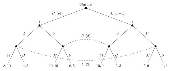
A pure strategy for player 1 is a pair \(XY\) giving his action as the \(H\) type and as the \(L\) type, so \(S_1 = \{UU, UD, DU, DD\}\). A pure strategy for player 2 is a pair giving her action after \(U\) and after \(D\), so \(S_2 = \{MM, MB, BM, BB\}\). Let \(\mu_U\) and \(\mu_D\) denote player 2’s belief that player 1 is the \(H\) type after observing \(U\) and \(D\) respectively. A useful preliminary: after observing \(U\) with belief \(\mu_U\) on \(H\), player 2’s expected profit from \(M\) is \(10\mu_U\) and from \(B\) is \(5\mu_U + 3(1-\mu_U) = 3 + 2\mu_U\), so she is indifferent at \(10\mu_U = 3 + 2\mu_U\), i.e. \(\mu_U = \tfrac38\); thus \[ B \text{ is optimal after } U \iff \mu_U \le \tfrac38 . \tag{5.3}\]
Equilibria for \(p = \tfrac14\)
We enumerate player 1’s four pure strategies.
\(UD\) gives no PBE. If \(UD\) is played, both messages are on the path and consistency forces \(\mu_U = 1\) (only \(H\) chose \(U\)) and \(\mu_D = 0\) (only \(L\) chose \(D\)). Sequential rationality then makes player 2 choose \(M\) after \(U\) and \(B\) after \(D\), i.e. play \(MB\). But against \(MB\) the \(L\) type earns only \(1\) as a blue-collar worker after \(D\), whereas deviating to \(U\) would make him a manager worth \(10\). The \(L\) type deviates, so \(UD\) supports no PBE.
\(DU\) gives the separating PBE \((DU, BM)\). If \(DU\) is played, consistency forces \(\mu_U = 0\) (only \(L\) chose \(U\)) and \(\mu_D = 1\) (only \(H\) chose \(D\)). Sequential rationality then makes player 2 play \(B\) after \(U\) and \(M\) after \(D\), i.e. \(BM\). Given \(BM\), neither type wishes to deviate: the \(H\) type earns \(8\) (\(=10-2\)) as a manager and would earn only \(6\) as a blue-collar worker by switching to \(U\); the \(L\) type earns \(6\) as a blue-collar worker and would earn only \(5\) (\(=10-5\)) as a manager by switching to \(D\). Hence \[ (DU,\ BM) \text{ with beliefs } (\mu_U = 0,\ \mu_D = 1) \] is a perfect Bayesian equilibrium. This is a separating equilibrium: the two types choose different actions, so player 2 perfectly infers the type — after \(U\) she knows it is \(L\), and after \(D\) she knows it is \(H\).
\(UU\) gives the pooling PBE \((UU, BB)\). If both types choose \(U\), then \(U\) is on the path and consistency forces \(\mu_U = p = \tfrac14\). By Equation 5.3, since \(\tfrac14 \le \tfrac38\), player 2 optimally plays \(B\) after \(U\) (manager profit \(10\cdot\tfrac14 = 2.5\) against blue-collar profit \(3 + 2\cdot\tfrac14 = 3.5\)). For no type to want to deviate to \(D\), player 2 must also choose \(B\) after \(D\); this is sequentially rational provided \(\mu_D \le \tfrac38\), and since \(D\) is off the path, Requirement 3 lets us pick any such belief — e.g. \(\mu_D = 0\) (or indeed \(\mu_D = 0.01\)). Hence \[ (UU,\ BB) \text{ with beliefs } (\mu_U = \tfrac14,\ \mu_D = 0) \] is a perfect Bayesian equilibrium. This is a pooling equilibrium: both types choose the same action, revealing nothing.
\(DD\) gives no PBE. If both types choose \(D\), then \(D\) is on the path and consistency forces \(\mu_D = p = \tfrac14\). By the same arithmetic as Equation 5.3 (with \(D\) in place of \(U\)), player 2 optimally plays \(B\) after \(D\). But then the \(L\) type, who pays the high cost \(c_L = 5\) for the degree only to remain a blue-collar worker, strictly prefers to deviate to \(U\) regardless of what player 2 does after \(U\). So \(DD\) supports no PBE.
No mixed-strategy PBE either. In any PBE the \(L\) type must play \(U\): were the \(L\) type ever to incur the cost of \(D\), the foregoing arguments show he would rather not. Suppose then the \(H\) type mixes, playing \(U\) with probability \(q \in (0,1)\). Consistency gives \[ \mu_U = \frac{pq}{pq + (1-p)\cdot 1} < p = \tfrac14 , \] which by Equation 5.3 makes \(B\) strictly optimal after \(U\) — but then the \(H\) type is not indifferent between \(U\) and \(D\), contradicting that he mixes. So there is no other PBE, and in particular no mixed-strategy PBE.
In the separating equilibrium \((DU, BM)\), the degree credibly signals high ability even though education adds nothing to productivity. The high type can signal credibly because the low type does not want to imitate him. And the reason the low type stays put is not that he dislikes being a manager — he would love the manager’s wage, since \(w_M = 10 > 6 = w_B\). It is that the degree is simply too costly for him: \(c_L = 5 > 2 = c_H\). The differential cost of the signal is what makes it informative.
A mixed-strategy variant with \(p = \tfrac12\)
Raising the prior to \(p = \tfrac12\) admits a genuinely mixed PBE. As before, the \(L\) type plays \(U\). Suppose the \(H\) type plays \(U\) with probability \(q \in (0,1)\). Consistency gives \(\mu_D = 1\) (only \(H\) ever chooses \(D\)) and \[ \mu_U = \frac{pq}{pq + (1-p)} = \frac{q}{q+1} . \] For the \(H\) type to be willing to mix, player 2 must make him indifferent by mixing \(M\) and \(B\) with equal probability after \(U\); and for player 2 to be willing to mix, she must be indifferent after \(U\), which by Equation 5.3 requires \(\mu_U = \tfrac38\). Setting \(\tfrac{q}{q+1} = \tfrac38\) gives \(q = \tfrac35\). So the \(H\) type educates with probability \(\tfrac35\), player 2 randomises equally over \(M\) and \(B\) after \(U\), and \(\mu_U = \tfrac38\), \(\mu_D = 1\).
A finite signaling game: a continuum of equilibria
Signaling games need not have the clean separating/pooling dichotomy of the education model; mixed equilibria can form a continuum. Consider the abstract game of Figure 5.5. Nature draws a sender type \(t_1\) or \(t_2\), each with probability \(\tfrac12\); the sender sends message \(b\) or \(q\); the receiver, observing only the message, responds with \(f\) or \(r\). Payoffs \((\text{sender}, \text{receiver})\) are
| type, message | \(f\) | \(r\) |
|---|---|---|
| \(t_1,\ b\) | \(1,\,1\) | \(-1,\,0\) |
| \(t_1,\ q\) | \(-2,\,1\) | \(0,\,0\) |
| \(t_2,\ b\) | \(-2,\,-1\) | \(0,\,0\) |
| \(t_2,\ q\) | \(-3,\,-1\) | \(-1,\,0\) |
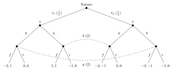
Look for an equilibrium in which both messages are sent with positive probability. Let \(\sigma(t_1), \sigma(t_2) \in (0,1)\) be the probabilities that each type sends \(b\), and let \(\tau(b), \tau(q)\) be the receiver’s probabilities of playing \(f\) after each message. For each sender type to mix, it must be indifferent between the two messages: \[ \underbrace{\tau(b) - \big(1 - \tau(b)\big)}_{t_1 \text{ from } b} = \underbrace{-2\tau(q)}_{t_1 \text{ from } q}, \qquad \underbrace{-2\tau(b)}_{t_2 \text{ from } b} = \underbrace{-3\tau(q) - \big(1 - \tau(q)\big)}_{t_2 \text{ from } q}. \] These two equations solve to \(\tau(b) = \tfrac12\) and \(\tau(q) = 0\). For the receiver to randomise after \(b\) (i.e. \(\tau(b)=\tfrac12\)) he must be indifferent there, which requires the posterior \(\mu_b = \Prob(t_1 \mid b) = \tfrac12\). By Bayes’ rule (Definition 5.2), \[ \mu_b = \frac{\tfrac12\,\sigma(t_1)}{\tfrac12\,\sigma(t_1) + \tfrac12\,\sigma(t_2)} = \tfrac12 \iff \sigma(t_1) = \sigma(t_2), \] and then the posterior after \(q\) is also \(\mu_q = \tfrac12\), which makes playing \(r\) (\(\tau(q)=0\)) a best response. Every common value \(\sigma(t_1) = \sigma(t_2) = \sigma \in (0,1)\) therefore supports a perfect Bayesian equilibrium: \[ \sigma(t_1) = \sigma(t_2) = \sigma \in (0,1), \quad \tau(b) = \tfrac12, \quad \tau(q) = 0, \quad \mu_b = \mu_q = \tfrac12 . \] There is a whole continuum of equilibria, indexed by \(\sigma\) — a reminder that perfect Bayesian equilibrium, like Nash equilibrium before it, need not pin down a unique prediction.
5.5 Refinement: the intuitive criterion
The pooling equilibrium \((UU, BB)\) survives only because Requirement 3 lets player 2 hold an arbitrary belief off the path: she may believe that a deviator to \(D\) is very likely the \(L\) type, which justifies punishing the deviation with \(B\). But is that belief reasonable? The Cho–Kreps intuitive criterion sharpens PBE by ruling out off-path beliefs that no rational type would induce.
Fix a subset of types \(\hat\Theta \subset \Theta\) and an action \(a_1\) for player 1. Let \(BR_2(\hat\Theta, a_1) \subset A_2\) be the set of player-2 best responses when player 2 sees \(a_1\) and her belief puts positive probability only on types in \(\hat\Theta\): \[ BR_2(\hat\Theta, a_1) \equiv \bigcup_{\mu \in \Delta(\hat\Theta)} \argmax_{a_2 \in A_2} \sum_{\theta \in \hat\Theta} \mu(\theta)\, v_2(a_1, a_2, \theta) . \] Given a PBE with equilibrium payoffs \(U(\theta)\), let \(D(a_1)\) be the set of types that have no incentive to deviate to \(a_1\), even under the most favourable response: \[ D(a_1) \equiv \Big\{\, \theta \in \Theta \ \Big|\ U(\theta) > \max_{a_2 \in BR_2(\Theta, a_1)} v_1(a_1, a_2, \theta) \,\Big\} . \]
Definition 5.4 (Failing the intuitive criterion (Cho–Kreps)) A PBE \(\sigma\) of a signaling game fails the intuitive criterion if there exists a type \(\theta\) and an off-path action \(a_1\) such that \[ U(\theta) < \min_{a_2 \in BR_2(\Theta \sm D(a_1),\, a_1)} v_1(a_1, a_2, \theta) . \]
The story is this: type \(\theta\) deviates to \(a_1\) and points out that no type in \(D(a_1)\) would ever have an incentive to make this deviation, so player 2 should believe the deviator is one of \(\Theta \sm D(a_1)\). Convinced, she responds with some action in \(BR_2(\Theta \sm D(a_1), a_1)\) — and type \(\theta\) profits from the deviation no matter which such response she chooses. Whenever such a \(\theta\) and \(a_1\) exist, the equilibrium is judged unreasonable.
The pooling equilibrium fails. Return to \((UU, BB)\) with off-path belief placing high probability on \(L\) after \(D\) (so that \(B\) is justified). Consider the deviation \(a_1 = D\). The relevant best-response sets are \[ BR_2(\{H,L\}, D) = \{M, B\}, \quad BR_2(\{H\}, D) = \{M\}, \quad BR_2(\{L\}, D) = \{B\}. \] Who would never deviate to \(D\)? The \(L\) type: by deviating he could earn at most \(5\) (manager wage \(10\) minus cost \(c_L = 5\)), whereas in equilibrium he earns \(6\) as a blue-collar undergraduate. So \(L \in D(D)\), and in fact \(D(D) = \{L\}\). The \(H\) type can therefore argue: “only \(H\) would ever choose \(D\).” With the \(L\) type ruled out, \(BR_2(\Theta \sm D(D), D) = BR_2(\{H\}, D) = \{M\}\), and the \(H\) type’s payoff from \(D\) would then be \(v_1(D, M, H) = w_M - c_H = 10 - 2 = 8\). Comparing with his equilibrium payoff \(U(H) = 6\), \[ U(H) = 6 < 8 = \min_{a_2 \in BR_2(\Theta \sm D(D),\, D)} v_1(D, a_2, H) . \] The inequality of Definition 5.4 holds, so \((UU, BB)\) fails the intuitive criterion and is discarded. The separating equilibrium \((DU, BM)\), by contrast, survives.
5.6 Cheap talk
In a cheap-talk game, due to Crawford and Sobel, the sender’s message has no direct effect on payoffs — it is costless and payoff-irrelevant. This is the polar opposite of signaling, where the signal is costly. The question becomes whether any information can be credibly transmitted when talk is free.
The structure is as follows. Nature draws a type \(\theta \in \Theta\) from a known distribution \(p\). The sender (player 1) learns \(\theta\) and sends a message \(a_1 \in A_1\); the receiver (player 2) observes \(a_1\) and chooses an action \(a_2 \in A_2\). Payoffs \(v_1(a_2, \theta)\) and \(v_2(a_2, \theta)\) depend on the receiver’s action and the type, not on the message. Strategies are \(\sigma_1: \Theta \to \Delta(A_1)\) for the sender and \(\sigma_2: A_1 \to \Delta(A_2)\) for the receiver, and player 2 holds beliefs \(\mu: A_1 \to \Delta(\Theta)\), with \(\mu(\cdot \mid a_1)\) the posterior over types after message \(a_1\). A PBE is a pair \((\sigma_1^*, \sigma_2^*)\) and beliefs \(\mu\) satisfying:
- Sender optimality: for each \(\theta\), \[ \sigma_1^*(\theta) \in \argmax_{\sigma_1 \in \Sigma_1} \sum_{a_1 \in A_1} \sigma_1(a_1)\, v_1\big(\sigma_2^*(a_1), \theta\big); \]
- Receiver optimality: for each \(a_1\), \[ \sigma_2^*(a_1) \in \argmax_{\sigma_2 \in \Sigma_2} \sum_{\theta \in \Theta} \mu(\theta \mid a_1)\, v_2(\sigma_2, \theta); \]
- Consistency (Bayes’ rule on path): if \(a_1\) is on the path, \[ \mu(\theta \mid a_1) = \frac{p(\theta)\,\sigma_1^*(\theta)[a_1]} {\sum_{\theta'} p(\theta')\,\sigma_1^*(\theta')[a_1]} . \]
The uniform–quadratic example
Take \(\Theta = [0,1]\) with a uniform prior, \(A_1 = [0,1]\), and \(A_2 = \R\). The payoffs are \[ v_2(a_2, \theta) = -(a_2 - \theta)^2, \qquad v_1(a_2, \theta) = -(a_2 - b - \theta)^2, \] with a constant bias \(b > 0\). For each \(\theta\), the receiver most prefers \(a_2 = \theta\) while the sender most prefers \(a_2 = b + \theta\): the sender always wants the receiver to choose higher than the receiver would, and \(b\) measures the conflict of interest. We render the four results as “Claims,” since Quarto has no claim environment.
Claim 5.1 (No fully revealing PBE). There is no PBE in which the message fully reveals the type — i.e. no equilibrium such that for all \(\theta\), \(a_1 \in \operatorname{supp}\sigma_1^*(\theta)\) implies \(\mu(\theta \mid a_1) = 1\). In particular the truthful strategy \(s_1(\theta) = \theta\) cannot appear in any equilibrium.
Proof. Suppose, for contradiction, such an equilibrium exists. Consider \(\theta = 0\) and pick any \(a_1 \in \operatorname{supp}\sigma_1^*(0)\). Since \(\mu(0 \mid a_1) = 1\), receiver optimality gives \(s_2^*(a_1) = 0\), so the type-\(0\) sender earns \(-(0 - b - 0)^2 = -b^2\).
- If \(b \in (0,1]\), pick any \(a_1' \in \operatorname{supp}\sigma_1^*(b)\). Since \(\mu(b \mid a_1') = 1\), \(s_2^*(a_1') = b\), so deviating to \(a_1'\) would give the type-\(0\) sender \(-(b - b - 0)^2 = 0 > -b^2\), a profitable deviation.
- If \(b > 1\), pick any \(a_1' \in \operatorname{supp}\sigma_1^*(1)\). Since \(\mu(1 \mid a_1') = 1\), \(s_2^*(a_1') = 1\), so deviating gives \(-(1 - b - 0)^2 > -(0 - b - 0)^2\) (as \(|1-b| < b\) when \(b > 1\)), again profitable.
Either way the type-\(0\) sender has a profitable deviation, contradicting equilibrium. \(\square\)
Claim 5.2 (A babbling equilibrium always exists). There is always a babbling PBE in which the message reveals nothing and the receiver chooses the action that maximises his expected payoff under the prior.
Proof. By construction. Take \(s_1^*(\theta) = 0\) for all \(\theta\), \(s_2^*(a_1) = \tfrac12\) for all \(a_1\), and \(\mu(\cdot \mid a_1) = p\) for all \(a_1\). Since \(s_2^*\) is constant, the sender’s action cannot influence the receiver, so no sender type has a profitable deviation. Given the prior belief, the receiver’s expected payoff after any message is \(\int_0^1 -(s_2 - \theta)^2\, d\theta\), which is maximised at \(s_2 = \tfrac12 = \E[\theta]\), the mean of the uniform prior. Finally, \(a_1 = 0\) is the only on-path message and conveys no information, so \(\mu(\cdot \mid 0) = p\) is consistent. \(\square\)
The interesting case lies between full revelation and babbling: a two-message equilibrium in which the sender partitions the type space into two intervals.
Claim 5.3 (Structure of a two-message equilibrium). Suppose the sender uses only two messages: there is a set \(L \subset \Theta\) and messages \(a_1, a_1'\) with \(s_1(\theta) = a_1\) for \(\theta \in L\) and \(s_1(\theta) = a_1'\) otherwise, and (without loss) \(s_2(a_1) < s_2(a_1')\). If this profile together with some consistent beliefs is a PBE, then there is a cutoff \(\theta^* \in (0,1)\) such that
the sender uses a cutoff rule, \(s_1(\theta) = a_1\) if \(\theta < \theta^*\) and \(s_1(\theta) = a_1'\) if \(\theta > \theta^*\);
type \(\theta^*\) is indifferent between the two messages;
\(s_2(a_1) = \dfrac{\theta^*}{2}\) and \(s_2(a_1') = \dfrac{1+\theta^*}{2}\).
Proof. Suppose \(s_1(\theta) = a_1\) for some interior \(\theta\). Sender optimality gives \[ -(s_2(a_1) - b - \theta)^2 \ge -(s_2(a_1') - b - \theta)^2 , \] equivalently \[ 2\big(s_2(a_1) - s_2(a_1')\big)\theta \ge (s_2(a_1) - b)^2 - (s_2(a_1') - b)^2 . \] Since \(s_2(a_1) - s_2(a_1') < 0\), the left-hand side strictly increases as \(\theta\) decreases, so for any \(\theta' < \theta\) the inequality is strict: \[ -(s_2(a_1) - b - \theta')^2 > -(s_2(a_1') - b - \theta')^2 , \] whence \(s_1(\theta') = a_1\) for all \(\theta' < \theta\). Symmetrically, if \(s_1(\theta) = a_1'\) then \(s_1(\theta') = a_1'\) for all \(\theta' > \theta\). Hence there is a cutoff \(\theta^* \in (0,1)\) with the stated form. Because the sender weakly prefers \(a_1\) below \(\theta^*\) and \(a_1'\) above it, continuity gives indifference exactly at \(\theta^*\): \[ -(s_2(a_1) - b - \theta^*)^2 = -(s_2(a_1') - b - \theta^*)^2 . \] For the receiver: after \(a_1\) the posterior is uniform on \([0, \theta^*]\), so the optimal action is its mean \(s_2(a_1) = \tfrac{\theta^*}{2}\); after \(a_1'\) the posterior is uniform on \([\theta^*, 1]\), so \(s_2(a_1') = \tfrac{1+\theta^*}{2}\). \(\square\)
Claim 5.4 (A two-message PBE exists iff the bias is small). A two-message PBE exists if and only if \(b < \tfrac14\), in which case the cutoff is \(\theta^* = \tfrac12 - 2b\).
Proof. (Necessity.) By Claim 5.3, type \(\theta^*\) must be indifferent, and substituting \(s_2(a_1) = \tfrac{\theta^*}{2}\) and \(s_2(a_1') = \tfrac{1+\theta^*}{2}\) gives \[ -\Big(\tfrac{\theta^*}{2} - b - \theta^*\Big)^2 = -\Big(\tfrac{1+\theta^*}{2} - b - \theta^*\Big)^2 . \] Taking absolute values, \(\big|{-\tfrac{\theta^*}{2} - b}\big| = \big|\tfrac{1-\theta^*}{2} - b\big|\). The two inside terms cannot be equal in the relevant range, so we set one equal to minus the other: \[ \tfrac{\theta^*}{2} + b = \tfrac{1-\theta^*}{2} - b \implies \theta^* = \tfrac12 - 2b . \] This lies in \((0,1)\) iff \(b < \tfrac14\); if \(b \ge \tfrac14\) no admissible cutoff exists, so no two-message PBE exists.
(Sufficiency.) If \(b < \tfrac14\), set \(\theta^* = \tfrac12 - 2b \in (0,1)\). Then the strategies \[ s_1(\theta) = \begin{cases} a_1, & \theta \le \theta^*,\\[2pt] a_1', & \theta > \theta^*, \end{cases} \qquad s_2(a_1'') = \begin{cases} \dfrac{\theta^*}{2}, & a_1'' \ne a_1',\\[6pt] \dfrac{1+\theta^*}{2}, & a_1'' = a_1', \end{cases} \] together with beliefs \(\mu(\cdot \mid a_1'')\) uniform on \([0, \theta^*]\) when \(a_1'' \ne a_1'\) and uniform on \([\theta^*, 1]\) when \(a_1'' = a_1'\), satisfy all three PBE conditions. \(\square\)
The lessons of the cheap-talk model are stark. With any bias \(b > 0\), information can never be fully transmitted (Claim 5.1). A completely uninformative babbling equilibrium always exists (Claim 5.2). But when the bias is small enough — \(b < \tfrac14\) — partial communication is possible through a two-message, interval-partition equilibrium (Claims 5.3–5.4). Whether still finer communication is feasible (three-, four-, …, \(M\)-message equilibria) is the natural next question.
5.7 Chapter summary
- With incomplete information, sequential play creates information sets that prevent the tree from splitting into proper subgames, so Nash \(=\) SPE and subgame perfection “has no bite” — motivating a finer concept.
- A perfect Bayesian equilibrium (Definition 5.3) augments a Bayesian Nash equilibrium with a system of beliefs \(\mu\) (Definition 5.2) and imposes four requirements: beliefs exist; on-path beliefs obey Bayes’ rule (\(\mu(x) = \Prob^{\sigma^*}(x)/\Prob^{\sigma^*}(h)\)); off-path beliefs are unrestricted; and strategies are sequentially rational given beliefs.
- When a BNE reaches every information set, the consistent belief system is unique and the BNE is automatically a PBE (Proposition 5.1).
- In signaling games, an informed sender’s costly action can credibly convey its type. In Spence’s education model, the degree is completely unproductive yet signals high ability in the separating equilibrium \((DU, BM)\), because imitation is too costly for the low type (\(c_L = 5 > c_H = 2\)); there is also a pooling equilibrium \((UU, BB)\) revealing nothing, and (at \(p = \tfrac12\)) a mixed equilibrium with the high type educating with probability \(\tfrac35\).
- The intuitive criterion (Definition 5.4) refines PBE by deleting off-path beliefs on types \(D(a_1)\) that would never deviate; the pooling equilibrium fails it because \(U(H) = 6 < 8\), while the separating equilibrium survives.
- In cheap talk, the message is costless and payoff-irrelevant: full revelation is impossible for any bias (Claim 5.1), babbling always exists (Claim 5.2), and a partially informative two-message equilibrium with cutoff \(\theta^* = \tfrac12 - 2b\) exists exactly when \(b < \tfrac14\) (Claims 5.3–5.4).