2 Static Games with Complete Information

\[ \newcommand{\E}{\mathbb{E}} \newcommand{\R}{\mathbb{R}} \newcommand{\Prob}{\mathbb{P}} \newcommand{\BR}{\operatorname{BR}} \newcommand{\eps}{\varepsilon} \newcommand{\given}{\,\vert\,} \newcommand{\argmax}{\operatorname*{arg\,max}} \newcommand{\argmin}{\operatorname*{arg\,min}} \newcommand{\sm}{\setminus} \newcommand{\defeq}{\equiv} \]

This chapter develops the workhorse model of game theory: the normal-form game, in which players choose once and simultaneously, and everything about the game is common knowledge. We build up the central solution concept — Nash equilibrium — through a sequence of weaker ideas (dominance, iterated elimination, best response), then put it to work on Cournot, Bertrand and electoral competition, and finally extend it to mixed strategies so that an equilibrium is guaranteed to exist.

2.1 Normal-form games

Definition 2.1 (Normal-form game) A normal-form game consists of three ingredients:

a finite set of players $N = \{1, 2, \dots, n\}$;
for each player $i$, a strategy space $S_i$ — the set of strategies available to $i$;
for each player $i$, a payoff function $v_i : S_1 \times \cdots \times S_n \to \R$.

We write the game as the triple $\Gamma = \big(N, \{S_i\}_{i=1}^n, \{v_i\}_{i=1}^n\big)$.

An element $s_i \in S_i$ is a strategy; a vector $s = (s_1, \dots, s_n) \in S_1 \times \cdots \times S_n$ is a strategy profile. The game is finite if every $S_i$ has finitely many elements.

It is convenient to single out one player and bundle the rest. Fixing player $i$, write \[ s_{-i} \defeq (s_1, \dots, s_{i-1}, s_{i+1}, \dots, s_n), \qquad S_{-i} \defeq \textstyle\prod_{j \ne i} S_j , \] so that a profile decomposes as $s = (s_i, s_{-i})$ and a payoff as $v_i(s_i, s_{-i})$. Read $s_{-i}$ as “what everyone other than $i$ does”.

A two-player finite game is displayed as a bimatrix: player 1 chooses the row, player 2 the column, and each cell lists $(\text{payoff to } 1, \text{payoff to } 2)$.

Three examples

The Prisoner’s Dilemma. Two suspects are interrogated separately. Each can deny ($D$) or confess ($C$). If both deny they get 2 years each; if one confesses while the other denies, the confessor gets 1 year and the denier 5; if both confess, 4 years each. Payoffs are minus the years served.

Table 2.1: The Prisoner’s Dilemma (rows = suspect 1, columns = suspect 2).

	$D$	$C$
$D$	$-2,\,-2$	$-5,\,-1$
$C$	$-1,\,-5$	$-4,\,-4$

Rock–paper–scissors. Each player picks $R$, $P$ or $S$; the loser pays the winner $1, ties pay nothing. This is a zero-sum game (the payoffs in every cell sum to zero).

Table 2.2: Rock–paper–scissors.

	$R$	$P$	$S$
$R$	$0,\,0$	$-1,\,1$	$1,\,-1$
$P$	$1,\,-1$	$0,\,0$	$-1,\,1$
$S$	$-1,\,1$	$1,\,-1$	$0,\,0$

Voting on a new agenda. Three voters $N=\{1,2,3\}$ each choose $Y$ (yes), $N$ (no) or $A$ (abstain). A new policy passes under majority rule iff strictly more than half of those who vote (do not abstain) choose $Y$. Relative to the status quo (payoff $0$ to all), the new policy is worth $+1$ to voters 1 and 2 and $-1$ to voter 3. This is a three-player game, so it takes three bimatrices (one per choice of voter 3) to display — a first hint that the matrix representation does not scale.

2.2 Dominance

The most basic principle is that a rational player never plays a strategy that is always worse than some alternative.

Definition 2.2 (Strictly dominated strategy) A strategy $s_i' \in S_i$ is strictly dominated by $s_i \in S_i$ if it does strictly worse no matter what the opponents do: \[ v_i(s_i, s_{-i}) > v_i(s_i', s_{-i}) \qquad \text{for all } s_{-i} \in S_{-i}. \]

Definition 2.3 (Strictly dominant strategy) A strategy $s_i \in S_i$ is strictly dominant for player $i$ if it strictly dominates every other strategy: for all $s_i' \ne s_i$, \[ v_i(s_i, s_{-i}) > v_i(s_i', s_{-i}) \qquad \text{for all } s_{-i} \in S_{-i}. \]

Definition 2.4 (Strictly dominant strategy equilibrium) A profile $s \in S$ is a strictly dominant strategy equilibrium if $s_i$ is a strictly dominant strategy for every player $i$.

In the Prisoner’s Dilemma, confessing strictly dominates denying for each suspect: whatever the other does, confessing shaves a year off the sentence. So $(C,C)$ is a strictly dominant strategy equilibrium — a remarkably sharp prediction that requires only that each player be rational, with no assumption about beliefs.

Lemma 2.1 (Uniqueness of a dominant strategy) If player $i$ has a strictly dominant strategy, it is unique.

Proposition 2.1 (Uniqueness of the dominant-strategy equilibrium) If a game has a strictly dominant strategy equilibrium $s$, then $s$ is its unique dominant strategy equilibrium.

Both follow immediately from the strict inequalities in the definitions (if two strategies were each dominant, each would have to strictly beat the other — a contradiction), and the slides leave them as quick exercises.

The dominant-strategy prediction can be collectively self-defeating.

Definition 2.5 (Pareto dominance and Pareto optimality) A profile $s$ Pareto dominates $s'$ if $v_i(s) \ge v_i(s')$ for all $i$, with strict inequality for at least one $i$. A profile is Pareto optimal (or Pareto efficient) if no other profile Pareto dominates it.

In the Prisoner’s Dilemma the equilibrium $(C,C)$ pays $(-4,-4)$, yet $(D,D)$ pays $(-2,-2)$ and Pareto dominates it. Rational individual behaviour leads to a collectively worse outcome — the defining tension of the game, and the reason it is the canonical model of why cooperation is hard to sustain.

2.3 Iterated elimination of strictly dominated strategies

Most games have no dominant strategy. But we can still apply the logic of dominance repeatedly: if I am rational I delete my dominated strategies; if I know you are rational I can delete yours; if I know that you know that I am rational I can delete more of mine; and so on. The “and so on” needs a name.

Definition 2.6 (Common knowledge) An event $E$ is common knowledge if everyone knows $E$, everyone knows that everyone knows $E$, everyone knows that everyone knows that everyone knows $E$, and so on ad infinitum.

The IESDS procedure

Set $S_i^0 = S_i$ for every player. Given the reduced game with strategy sets $\{S_i^k\}$: if some player has a strictly dominated strategy in this reduced game, delete (at least) those strategies to obtain $\{S_i^{k+1}\}$; if no player has a strictly dominated strategy, stop. A strategy in $S_i^* = \bigcap_{k\ge 0} S_i^k$ is said to survive iterated elimination of strictly dominated strategies (IESDS), and a surviving profile is called an iterated-elimination equilibrium.

Consider the game

Table 2.3: An IESDS example.

	$L$	$C$	$R$
$U$	$4,\,3$	$5,\,1$	$6,\,2$
$M$	$2,\,1$	$8,\,4$	$3,\,6$
$D$	$3,\,0$	$9,\,6$	$2,\,8$

For player 2, $C$ is strictly dominated (by $R$, say); delete it. In the resulting $3\times2$ game, $M$ and $D$ become strictly dominated for player 1 by $U$; delete them. Now player 2 prefers $L$ to $R$; delete $R$. Only $(U,L)$ survives. The prediction is unique — but note what it rests on: not just that both players are rational, but that this is common knowledge. The third deletion uses “player 2 knows that player 1 knows that player 2 is rational.”

Proposition 2.2 (Dominant equilibria survive IESDS) If $s$ is a strictly dominant strategy equilibrium, then for every player $s_i$ is the unique survivor of IESDS.

Proof. For each player $i$, every other strategy $s_i' \ne s_i$ is strictly dominated by $s_i$ (that is what dominance means), so all of them are deleted in the very first round, leaving $s_i$ alone. $\square$

Order independence. For a finite game the procedure terminates, and the surviving set $S^*$ does not depend on the order in which dominated strategies are removed — it is enough that some dominated strategy be deleted each round. For infinite games the process may not terminate, and to keep the answer order-independent one insists that all currently-dominated strategies be deleted in each round.

IESDS in the Cournot duopoly

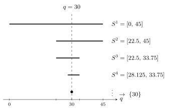
Two firms choose quantities $q_1, q_2 \ge 0$. The market price is $P(Q) = \max\{100 - Q, 0\}$ with $Q = q_1 + q_2$, and each firm has constant marginal cost $10$, so \[ v_i(q_i, q_j) = \max\{100 - q_i - q_j,\, 0\}\, q_i - 10\, q_i . \] Let $\phi(q) = \tfrac{90 - q}{2}$ be a firm’s profit-maximising quantity when its rival produces $q$. IESDS shrinks the strategy space step by step:

Any $q_i > 45$ is strictly dominated by $q_i = 45$, so $S^1 = [0, 45]$.
Given $q_j \in [0,45]$, the best reply lies in $[22.5, 45]$, and any $q_i < 22.5$ is now strictly dominated by $22.5$, so $S^2 = [22.5, 45]$.
Iterating, $S^3 = [22.5, 33.75]$, $S^4 = [28.125, 33.75]$, and so on.

The endpoints are successive iterates of $\phi$ starting from $0$, and since $\phi^{(k)}(0) \to 30$, the intervals collapse: $S_i^* = \bigcap_{k} S_i^k = \{30\}$ (Figure 2.1). IESDS alone pins down the Cournot quantity $q_1 = q_2 = 30$ — no equilibrium concept required yet.

Figure 2.1: IESDS in the Cournot duopoly: the surviving interval $[\underline q^{\,k}, \overline q^{\,k}]$ shrinks to the single point $q=30$ as the bounds chase the best-reply map $\phi(q)=(90-q)/2$.

2.4 Best response

Definition 2.7 (Best response) A strategy $s_i \in S_i$ is a best response to $s_{-i} \in S_{-i}$ if \[ v_i(s_i, s_{-i}) \ge v_i(s_i', s_{-i}) \qquad \text{for all } s_i' \in S_i . \]

Dominance and best response are two sides of the same coin.

Proposition 2.3 (Dominated strategies are never best responses) If $s_i$ is strictly dominated, then it is not a best response to any $s_{-i}$.

Proof. Suppose $s_i$ is strictly dominated by $s_i'$. Then for every $s_{-i}$ we have $v_i(s_i', s_{-i}) > v_i(s_i, s_{-i})$, so $s_i$ fails to maximise $i$’s payoff against any $s_{-i}$ and is never a best response. $\square$

Proposition 2.4 (Dominant strategies are the unique best response) If $s_i$ is strictly dominant, it is the unique best response to every $s_{-i}$.

This is immediate from the definitions. A subtler fact ties best response to the survivors of IESDS, and it is the first place where finiteness does real work.

Proposition 2.5 (The IESDS survivor is a best response) In a finite game, if $s^*$ is the unique profile surviving IESDS, then $s_i^*$ is the unique best response to $s_{-i}^*$ for every player $i$.

Proof. Fix $i$ and suppose, for contradiction, that $s_i^*$ is not a best response to $s_{-i}^*$. Then some $s_i^1$ does strictly better: $v_i(s_i^1, s_{-i}^*) > v_i(s_i^*, s_{-i}^*)$. Since $s_i^*$ survives but $s_i^1$ does not, $s_i^1$ was deleted in some round — and a strategy is deleted only when strictly dominated, hence (against the surviving $s_{-i}^*$) there is some $s_i^2$ with $v_i(s_i^2, s_{-i}^*) > v_i(s_i^1, s_{-i}^*)$. But $s_i^2$ is also deleted, so there is $s_i^3$ beating it, and so on without end. This produces infinitely many distinct strategies, contradicting finiteness. Hence $s_i^*$ is a best response; that it is the unique best response follows from Proposition 2.3. $\square$

Important

The finiteness assumption is indispensable. The infinite chain $s_i^1, s_i^2, \dots$ is only a contradiction because $S_i$ is finite; for infinite games the conclusion can fail (a counterexample is left to the problem set).

When a strategy is the best response to several opponent profiles, it is cleaner to track the whole set of best responses as a function of $s_{-i}$. The best response correspondence $\BR_i : S_{-i} \rightrightarrows S_i$ is \[ \BR_i(s_{-i}) = \{\, s_i \in S_i : s_i \text{ is a best response to } s_{-i} \,\}. \] A correspondence is a set-valued map; we need it because a player may have several equally good replies.

2.5 Nash equilibrium

Definition 2.8 (Nash equilibrium) A profile $s^* = (s_1^*, \dots, s_n^*)$ is a Nash equilibrium if every player is best-responding to the others: for each $i$, \[ v_i(s_i^*, s_{-i}^*) \ge v_i(s_i, s_{-i}^*) \qquad \text{for all } s_i \in S_i, \] equivalently $s_i^* \in \BR_i(s_{-i}^*)$ for all $i$.

Definition 2.9 (Profitable deviation) Given a profile $s$, player $i$ has a profitable deviation if some $s_i'$ gives $v_i(s_i', s_{-i}) > v_i(s_i, s_{-i})$.

So a profile is a Nash equilibrium if and only if no player has a profitable deviation — the form in which equilibrium is usually checked. Conceptually, a Nash equilibrium combines two requirements:

rationality — each player chooses a best response to their belief about what the others do; and
consistency of beliefs — those beliefs are correct, i.e. each player correctly anticipates the others’ equilibrium strategies.

The concept is named for John Nash (Nobel Prize, 1994). It is the central prediction of non-cooperative game theory, and it relates cleanly to the earlier concepts.

Proposition 2.6 (A dominant equilibrium is the unique Nash equilibrium) A strictly dominant strategy equilibrium is the unique Nash equilibrium.

Proposition 2.7 (The IESDS survivor is the unique Nash equilibrium) In a finite game, if $s^*$ is the unique survivor of IESDS, it is the unique Nash equilibrium.

Proposition 2.8 (Nash equilibria survive IESDS) Every Nash equilibrium survives IESDS.

Proposition 2.6 follows from Proposition 2.4; Proposition 2.8 follows from Proposition 2.3 (an equilibrium strategy is a best response, hence never dominated, hence never deleted); and Proposition 2.7 combines Proposition 2.5 with Proposition 2.8.

Equilibrium is about strategies, not payoffs

Consider the variant of Battle of the Sexes with payoffs $(O,O)=(2,1)$, $(O,F)=(0,0)$, $(F,O)=(2,1)$, $(F,F)=(1,2)$. The profiles $(O,O)$ and $(F,O)$ give the same payoff $(2,1)$, yet $(O,O)$ is a Nash equilibrium while $(F,O)$ is not: at $(F,O)$, player 2 — facing $F$ — strictly prefers $F$ to $O$ and deviates. Equilibrium is a property of the strategy profile and the incentives it creates, not of the payoff it happens to deliver.

2.6 Applications

Coordination and “two kinds of societies”

Not every game has a unique equilibrium, and the multiplicity can be economically meaningful. In the Stag Hunt, two hunters each choose to hunt stag ($S$, which requires cooperation) or hare ($H$, which one can catch alone):

Table 2.4: The Stag Hunt.

	$S$	$H$
$S$	$5,\,5$	$0,\,3$
$H$	$3,\,0$	$3,\,3$

Both $(S,S)$ and $(H,H)$ are Nash equilibria. The cooperative equilibrium $(S,S)$ Pareto dominates $(H,H)$, yet $(H,H)$ can persist purely through pessimistic, self-fulfilling beliefs: if each expects the other to hunt hare, hunting hare is optimal. Two societies with identical fundamentals can settle into very different equilibria — a parable for why “norms of behaviour” matter. The driving game (both drive $L$ or both drive $R$, each a Nash equilibrium) makes the same point about social conventions.

Cournot competition

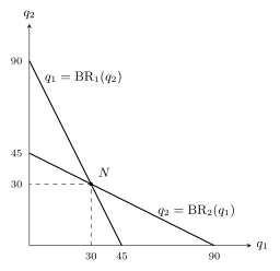
Generalise the duopoly of Section 2.3.1. Inverse demand is $P(Q) = \max\{a - bQ, 0\}$ and firm $i$ has constant marginal cost $c_i < a$, so \[ v_i(q_i, q_j) = \max\{a - b(q_i + q_j),\, 0\}\, q_i - c_i q_i . \] For a rival quantity $q_j < (a - c_i)/b$, the first-order condition $a - 2 b q_i - b q_j - c_i = 0$ gives the best-response function \[ \BR_i(q_j) = \max\!\left\{ \frac{a - b q_j - c_i}{2 b},\; 0 \right\}. \] A profile $(q_1^*, q_2^*)$ is a Nash equilibrium exactly when each firm is on its best-response curve. Solving the pair of linear equations, and watching for the non-negativity constraints, gives three regimes according to the signs of $a - 2c_1 + c_2$ and $a - 2c_2 + c_1$:

Interior (both expressions positive): \[ q_1^* = \frac{a - 2c_1 + c_2}{3b}, \qquad q_2^* = \frac{a - 2c_2 + c_1}{3b}. \]
One firm monopolises: if firm 2’s cost is so high that $a - 2c_2 + c_1 < 0$, then $q_2^* = 0$ and $q_1^* = (a - c_1)/(2b)$ (and symmetrically with the roles reversed).

Geometrically the two best-response lines slope downward and cross once (Figure 2.2). In the symmetric case $c_1 = c_2 = c$ the equilibrium is $q_1^* = q_2^* = (a - c)/(3b)$; with $a=100, b=1, c=10$ this is the quantity $30$ we already found by IESDS.

Figure 2.2: Cournot best responses. The two downward-sloping best-response lines $q_1=\BR_1(q_2)$ and $q_2=\BR_2(q_1)$ intersect at the unique interior Nash equilibrium $(q_1^*,q_2^*)$.

Bertrand competition

Now firms compete in prices rather than quantities. With identical marginal cost $c$, demand $Q(p) = \max\{a - p, 0\}$, and the lower-priced firm capturing the whole market (ties split it), \[ v_i(p_i, p_j) = \begin{cases} Q(p_i)(p_i - c), & p_i < p_j,\\[2pt] \tfrac12 Q(p_i)(p_i - c), & p_i = p_j,\\[2pt] 0, & p_i > p_j . \end{cases} \] The unique Nash equilibrium is $p_1^* = p_2^* = c$: price equals marginal cost, the competitive outcome, with just two firms. The argument is by elimination — any common price above $c$ invites a tiny undercut that steals the whole market, and below $c$ both firms lose money. Tellingly, the best-response correspondence is empty on the range $c < p_j \le p^m$ (the firm wants to undercut to $p_j - \eps$, but there is no smallest such price), which is exactly why one must argue by elimination rather than by intersecting best-response curves.

With asymmetric costs $c_1 < c_2$ the best-response correspondences never meet, and no pure-strategy Nash equilibrium exists: the low-cost firm always wants to sit just below the other’s price, so no profile is stable.

Electoral competition and the median voter

Two office-seeking candidates each choose a platform on a one-dimensional spectrum of policies $\{-50, \dots, 0, \dots, 50\}$. Each citizen votes for the nearer platform (splitting if indifferent), majority rule decides, and each candidate prefers winning to tying to losing. The unique Nash equilibrium has both candidates choose the median platform $0$: given that the opponent is at the median, any other platform loses, while matching ties. This is the discrete Hotelling model and its conclusion is the

Median Voter Theorem. When voters are arrayed on a single dimension and each prefers platforms nearer to their ideal point, the platform located at the median voter beats any other platform in a majority vote. Electoral competition drives both candidates to the centre.

2.7 Mixed strategies

Rock–paper–scissors and matching pennies have no Nash equilibrium in the strategies considered so far — whatever you do, your opponent would want to respond in a way that makes you want to change. The fix is to let players randomise.

Definition 2.10 (Mixed strategy) Let $S_i = \{s_{i1}, \dots, s_{im}\}$ be finite. A mixed strategy is a probability distribution $\sigma_i$ over $S_i$ — an element of the simplex $\Delta S_i = \big\{ \sigma_i : S_i \to [0,1] \,\big|\, \sum_{s_i \in S_i} \sigma_i(s_i) = 1 \big\}$. A pure strategy is the degenerate mixed strategy putting probability $1$ on a single action.

Definition 2.11 (Support) The support of $\sigma_i$ is the set of pure strategies it plays with positive probability, $\operatorname{supp}\sigma_i = \{ s_i : \sigma_i(s_i) > 0 \}$.

Players are expected-utility maximisers, so they evaluate a mixed profile by its expected payoff. If each player randomises independently, the profile $s = (s_1, \dots, s_n)$ occurs with probability $\prod_j \sigma_j(s_j)$, and \[ v_i(\sigma) = \sum_{s \in S} \Big( \prod_{j=1}^n \sigma_j(s_j) \Big) v_i(s) = \sum_{s_i \in S_i} \sigma_i(s_i)\, v_i(s_i, \sigma_{-i}) . \] The second form — a weighted average of the expected payoffs to $i$’s pure strategies — is the one we use constantly below.

2.8 Mixed-strategy Nash equilibrium

Definition 2.12 (Best response in mixed strategies) $\sigma_i$ is a best response to $\sigma_{-i}$ if $v_i(\sigma_i, \sigma_{-i}) \ge v_i(s_i, \sigma_{-i})$ for every pure $s_i \in S_i$. (Checking against pure strategies suffices: a mixture of weakly-worse pure strategies is weakly worse.)

The key computational tool is the following characterisation of when a mixture is optimal.

Lemma 2.2 (Indifference principle) A mixed strategy $\sigma_i$ is a best response to $\sigma_{-i}$ if and only if every pure strategy in $\operatorname{supp}\sigma_i$ is itself a best response to $\sigma_{-i}$. In particular, player $i$ is indifferent among all pure strategies in the support.

Proof. (If.) Suppose every $s_i \in \operatorname{supp}\sigma_i$ is a best response, so $v_i(s_i, \sigma_{-i}) \ge v_i(s_i', \sigma_{-i})$ for all $s_i'$. Averaging over the support with weights $\sigma_i(s_i)$, \[ v_i(\sigma_i, \sigma_{-i}) = \sum_{s_i \in \operatorname{supp}\sigma_i} \sigma_i(s_i)\, v_i(s_i, \sigma_{-i}) \ge \sum_{s_i \in \operatorname{supp}\sigma_i} \sigma_i(s_i)\, v_i(s_i', \sigma_{-i}) = v_i(s_i', \sigma_{-i}), \] so $\sigma_i$ is a best response.

(Only if.) Suppose $\sigma_i$ is a best response but some $s_i$ in its support is not. Let $\hat s_i$ be a best response, so $v_i(\hat s_i, \sigma_{-i}) > v_i(s_i, \sigma_{-i})$ while $v_i(\hat s_i, \sigma_{-i}) \ge v_i(s_i', \sigma_{-i})$ for all $s_i'$. Then, averaging over the support, \[ v_i(\hat s_i, \sigma_{-i}) = \sum_{s_i' \in \operatorname{supp}\sigma_i} \sigma_i(s_i')\, v_i(\hat s_i, \sigma_{-i}) > \sum_{s_i' \in \operatorname{supp}\sigma_i} \sigma_i(s_i')\, v_i(s_i', \sigma_{-i}) = v_i(\sigma_i, \sigma_{-i}), \] the strict inequality coming from the dominated term $s_i$. This contradicts $\sigma_i$ being a best response. Hence every support strategy is a best response, and they all attain the same maximal value — the indifference condition. $\square$

Definition 2.13 (Mixed-strategy Nash equilibrium) A mixed profile $\sigma^* = (\sigma_1^*, \dots, \sigma_n^*)$ is a Nash equilibrium if each $\sigma_i^*$ is a best response to $\sigma_{-i}^*$.

A practical consequence of Lemma 2.2: if a player genuinely mixes in equilibrium, the opponent’s probabilities must be tuned so as to make that player indifferent over their support. This is the “make-your-opponent- indifferent” recipe.

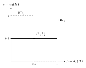
Matching pennies. With $\sigma_1(H) = p$ and $\sigma_2(H) = q$, player 1 is indifferent between $H$ and $T$ only when $q = \tfrac12$, and player 2 is indifferent only when $p = \tfrac12$. The best-response correspondences (Figure 2.3) are step functions that meet at the single point $(p,q) = (\tfrac12, \tfrac12)$: the unique equilibrium has each player mixing $\tfrac12 H + \tfrac12 T$.

Figure 2.3: Matching pennies. Player 1’s best-response correspondence (jumping at $q=\tfrac12$) and player 2’s (jumping at $p=\tfrac12$) meet only at $(\tfrac12,\tfrac12)$.

Rock–paper–scissors. A support argument rules out any equilibrium in which a player uses only one or two of the three actions; both players must randomise over all three. Indifference then forces the uniform mixture: the unique equilibrium is $\big(\tfrac13, \tfrac13, \tfrac13\big)$ for each player.

Battle of the Sexes. Beyond the two pure equilibria $(O,O)$ and $(F,F)$, there is a mixed equilibrium. Writing $\sigma_1(O)=p$, $\sigma_2(O)=q$: player 1’s indifference $2q = 1-q$ gives $q = \tfrac13$, and player 2’s indifference $p = 2(1-p)$ gives $p = \tfrac23$. The mixed equilibrium is $\big(\tfrac23 O + \tfrac13 F,\ \tfrac13 O + \tfrac23 F\big)$ — note that the players coordinate less often here than at either pure equilibrium.

2.9 Existence of equilibrium

Allowing mixed strategies is exactly what is needed to guarantee that an equilibrium always exists.

Theorem 2.1 (Nash, 1950) Every finite normal-form game has a Nash equilibrium, possibly in mixed strategies.

This is why we bothered with mixed strategies: matching pennies and rock–paper–scissors have no pure equilibrium, but the theorem assures us they have a mixed one — and we found it. (The proof, via Kakutani’s fixed-point theorem, is beyond our scope.)

2.10 Dominance and IESDS, revisited

A pure strategy can fail to be dominated by any other pure strategy yet still be dominated by a mixture.

Definition 2.14 (Dominance by a mixed strategy) A pure strategy $s_i$ is strictly dominated by the mixed strategy $\sigma_i \in \Delta S_i$ if \[ v_i(\sigma_i, s_{-i}) > v_i(s_i, s_{-i}) \qquad \text{for all } s_{-i} \in S_{-i}. \tag{2.1}\]

It makes no difference whether we test against the opponents’ pure profiles or all their mixtures: condition Equation 2.1 is equivalent to $v_i(\sigma_i, \sigma_{-i}) > v_i(s_i, \sigma_{-i})$ for all $\sigma_{-i} \in \Delta S_{-i}$, because the latter is just a convex average of the former.

For example, in

Table 2.5: A game requiring dominance by mixtures.

	$L$	$C$	$R$
$U$	$5,\,1$	$1,\,4$	$1,\,0$
$M$	$3,\,2$	$0,\,0$	$3,\,5$
$D$	$4,\,3$	$4,\,4$	$0,\,3$

no column is dominated by another column, but $L$ is strictly dominated by $\tfrac12 C + \tfrac12 R$; deleting $L$, then $U$ (now dominated by $\tfrac12 M + \tfrac12 R$), leaves the $\{M,D\}\times\{C,R\}$ subgame, whose equilibria are $(M,R)$, $(D,C)$ and the mixture $\big(\tfrac16 M + \tfrac56 D,\ \tfrac37 C + \tfrac47 R\big)$.

That this deletion is legitimate — that it removes no equilibrium — is the content of the final result.

Proposition 2.9 (IESDS preserves the equilibrium set) In a finite game, $\sigma^*$ is a Nash equilibrium of the original game if and only if it is a Nash equilibrium of the reduced game obtained by IESDS (allowing deletion by mixed strategies).

Proof. (If.) Let $\sigma^*$ be an equilibrium of the reduced game and suppose it is not one of the original. Then some player $i$ has a profitable deviation $s_i^1$, which must have been deleted (it is not in the reduced game). A deleted strategy is strictly dominated against the surviving opponents, so some $s_i^2$ beats $s_i^1$ against $\sigma_{-i}^*$; but $s_i^2$ is also deleted, so some $s_i^3$ beats it, and so on — infinitely many distinct strategies, contradicting finiteness.

(Only if.) No pure strategy in the support of an equilibrium mixed strategy is ever strictly dominated: if $s_i \in \operatorname{supp}\sigma_i^*$ were dominated by some $\sigma_i$, then averaging over $\sigma_{-i}^*$ would give $v_i(\sigma_i, \sigma_{-i}^*) > v_i(s_i, \sigma_{-i}^*)$, contradicting that $s_i$ is a best response (Lemma 2.2). So IESDS never deletes a support strategy, and $\sigma^*$ remains an equilibrium of the reduced game. $\square$

This is genuinely useful: IESDS first shrinks a large game, and Proposition 2.9 guarantees that hunting for equilibria in the small reduced game loses nothing.

2.11 Chapter summary

A normal-form game $\Gamma = (N, \{S_i\}, \{v_i\})$ specifies players, strategies and payoffs; two-player games are displayed as bimatrices.
Dominance gives the sharpest predictions where it applies: a rational player never plays a strictly dominated strategy, and the Prisoner’s Dilemma is solved by dominance alone — though its equilibrium is not Pareto optimal.
IESDS iterates this logic under common knowledge of rationality; for finite games the result is order-independent.
A Nash equilibrium is a profile in which everyone best-responds to everyone else — rationality plus correct beliefs. It nests the earlier concepts: dominant and IESDS solutions are Nash, and every Nash equilibrium survives IESDS.
Applications: Cournot (interior equilibrium $(a-2c_i+c_j)/3b$), Bertrand (price $=$ marginal cost; no equilibrium under asymmetric costs), and the median voter theorem in electoral competition.
Allowing mixed strategies, every finite game has an equilibrium (Theorem 2.1); they are computed via the indifference principle (Lemma 2.2).
IESDS by mixtures preserves the full set of equilibria (Proposition 2.9).

The next chapter lets players move in sequence, which both enriches the strategy space and exposes a weakness of Nash equilibrium — its tolerance of non-credible threats.

	\(D\)	\(C\)
\(D\)	\(-2,\,-2\)	\(-5,\,-1\)
\(C\)	\(-1,\,-5\)	\(-4,\,-4\)

	\(R\)	\(P\)	\(S\)
\(R\)	\(0,\,0\)	\(-1,\,1\)	\(1,\,-1\)
\(P\)	\(1,\,-1\)	\(0,\,0\)	\(-1,\,1\)
\(S\)	\(-1,\,1\)	\(1,\,-1\)	\(0,\,0\)

	\(L\)	\(C\)	\(R\)
\(U\)	\(4,\,3\)	\(5,\,1\)	\(6,\,2\)
\(M\)	\(2,\,1\)	\(8,\,4\)	\(3,\,6\)
\(D\)	\(3,\,0\)	\(9,\,6\)	\(2,\,8\)

	\(S\)	\(H\)
\(S\)	\(5,\,5\)	\(0,\,3\)
\(H\)	\(3,\,0\)	\(3,\,3\)

	\(L\)	\(C\)	\(R\)
\(U\)	\(5,\,1\)	\(1,\,4\)	\(1,\,0\)
\(M\)	\(3,\,2\)	\(0,\,0\)	\(3,\,5\)
\(D\)	\(4,\,3\)	\(4,\,4\)	\(0,\,3\)