3 Dynamic Games with Complete Information
\[ \newcommand{\E}{\mathbb{E}} \newcommand{\R}{\mathbb{R}} \newcommand{\Prob}{\mathbb{P}} \newcommand{\BR}{\operatorname{BR}} \newcommand{\eps}{\varepsilon} \newcommand{\given}{\,\vert\,} \newcommand{\argmax}{\operatorname*{arg\,max}} \newcommand{\argmin}{\operatorname*{arg\,min}} \newcommand{\sm}{\setminus} \newcommand{\defeq}{\equiv} \]
Most interesting strategic situations unfold over time: a chess match, a price war, a bargaining session, even an ordinary conversation. Players move in sequence, observe (some of) what has happened, and choose accordingly. The normal form of Chapter 2 collapses all of this into a single simultaneous choice of a strategy and so cannot represent who moves when, who sees what, or which threats are believable. This chapter develops the extensive form, which records the full dynamic structure as a game tree, and then refines Nash equilibrium to respect that structure. The central lesson is that Nash equilibrium of an extensive game — defined through its normal-form representation — is too permissive: it tolerates non-credible threats. Demanding sequential rationality at every point in the tree, formalised as subgame-perfect equilibrium, removes them. We close the first half with two applications: Stackelberg’s first-mover advantage and the Cuban-missile-crisis game of mutually assured destruction.
3.1 The extensive form
A normal-form game tells us the strategies and payoffs but says nothing about timing or information. The extensive form supplies exactly that missing structure. It is built on a game tree: a set of nodes connected by a precedence relation, with players assigned to the nodes at which decisions are made and payoffs attached to the final outcomes.
Definition 3.1 (Game tree) A game tree is a set of nodes \(x \in X\) together with a precedence relation \(x \succ x'\), read “\(x\) precedes \(x'\).” Every node has exactly one immediate predecessor, except for one special node, the root (or initial node), which has none. Nodes that do not precede any other node are terminal nodes, collected in the set \(Z\); they are the final outcomes of play. Every non-terminal node \(x\) is assigned to a player \(i(x)\), who chooses from an action set \(A_i(x)\); each action leads to a distinct successor node. Each terminal node \(z \in Z\) carries a payoff \(v_i(z) \in \R\) for every player \(i\). The game is finite if \(X\) is a finite set.
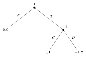
Consider the trust game of Figure 3.1. Player \(1\) moves first at the root: she may not trust (\(N\)), ending the game at the payoff \((0,0)\), or trust (\(T\)), passing the move to player \(2\). Player \(2\) then either cooperates (\(C\)), yielding \((1,1)\), or defects (\(D\)), yielding \((-1,2)\). Reading the tree from the root to a terminal node traces out one complete play of the game.
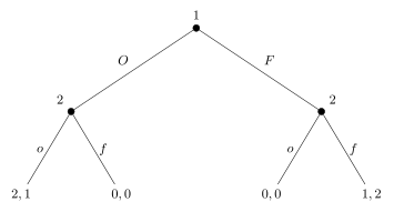
A second running example is the sequential-move Battle of the Sexes (Figure 3.2). Player \(1\) chooses \(O\) or \(F\); player \(2\) observes this choice and responds with \(o\) or \(f\). The four terminal payoffs are \((O,o)=(2,1)\), \((O,f)=(0,0)\), \((F,o)=(0,0)\) and \((F,f)=(1,2)\). Labelling the nodes makes the formal apparatus concrete: with \(X = \{x_0,x_1,x_2,x_3,x_4,x_5,x_6\}\), the root is \(x_0\) and the terminal set is \(Z = \{x_3,x_4,x_5,x_6\}\); the assignment is \(i(x_0)=1\) and \(i(x_1)=i(x_2)=2\); the action sets are \(A_1(x_0)=\{O,F\}\) and \(A_2(x_1)=A_2(x_2)=\{o,f\}\); and the payoffs are \(v_1(x_3)=2,\,v_1(x_4)=0,\,v_1(x_5)=0,\,v_1(x_6)=1\) for player \(1\) and \(v_2(x_3)=1,\,v_2(x_4)=0,\,v_2(x_5)=0,\,v_2(x_6)=2\) for player \(2\).
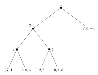
The tree can have more than two players and more than two moves per branch. Figure 3.3 shows a three-player game of perfect information. Player \(1\) moves at the root; her right branch ends immediately at \((2,0,-4)\), while her left branch hands the move to player \(2\). Player \(2\)’s left branch reaches a node owned by player \(3\) (with terminals \((1,7,4)\) and \((3,0,3)\)), and his right branch returns the move to player \(1\) at a second decision node of hers (with terminals \((2,2,5)\) and \((0,1,8)\)). Payoffs are now triples \((v_1,v_2,v_3)\).
So far each player, when called to move, has known exactly where in the tree she is. In general this need not be true: a player may be unable to distinguish among several of her decision nodes — for instance because she moves simultaneously with someone else and so cannot see their choice. Information sets encode precisely what a player can and cannot tell apart.
Definition 3.2 (Information sets) Each player \(i\) has a collection \(H_i\) of information sets \(h_i \in H_i\) that partition the nodes at which \(i\) moves, subject to:
- if \(h_i = \{x\}\) is a singleton, then \(i\), when moving at \(x\), knows he is at \(x\);
- if \(x \ne x'\) and both \(x, x' \in h_i\), then \(i\) cannot tell whether he is at \(x\) or at \(x'\);
- if \(x \ne x'\) and both \(x, x' \in h_i\), then \(A_i(x) = A_i(x')\).
Condition (3) is what makes the definition coherent: if the action sets at two indistinguishable nodes differed, the player could deduce his location simply by inspecting the menu of available actions, contradicting (2). We therefore write \(A_i(h_i)\) for the common action set on an information set \(h_i\).
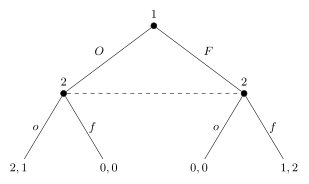
The simultaneous-move Battle of the Sexes (Figure 3.4) uses this device to model simultaneity inside a tree. The tree is identical to Figure 3.2, but player \(2\)’s two nodes \(x_1\) and \(x_2\) now lie in a single information set \(h_2 = \{x_1, x_2\}\), drawn as a dashed line joining them: player \(2\) must move without learning player \(1\)’s choice. Here \(H_1 = \{h_1\}\) with \(h_1 = \{x_0\}\) and \(H_2 = \{h_2\}\).
This dashed-line device is fully general: every normal-form game can be represented as an extensive-form game. Rock–paper–scissors, for instance, is drawn as player \(1\) choosing \(R\), \(P\) or \(S\), followed by player \(2\) choosing \(r\), \(p\) or \(s\) at a single information set spanning all three of player \(1\)’s possible nodes — so player \(2\) never learns player \(1\)’s choice, exactly as in the simultaneous game.
We maintain throughout a standing assumption that players never forget what they once knew.
Definition 3.3 (Perfect recall) A game has perfect recall if no player ever forgets information he previously knew, including his own past actions. We consider only games of perfect recall.
Games that violate perfect recall (a forgetful or “absent-minded” decision maker) are outside the scope of these notes. The remaining distinction concerns whether anyone is ever uncertain about the history of play.
Definition 3.4 (Perfect and imperfect information) An extensive-form game is a game of perfect information if every information set is a singleton. It is a game of imperfect information if some information set contains more than one node.
The trust game, the sequential Battle of the Sexes and the three-player tree are all games of perfect information. The simultaneous Battle of the Sexes and the extensive form of rock–paper–scissors are games of imperfect information.
3.2 Strategies
In a dynamic game a “strategy” must be a complete contingent plan: it has to specify what the player would do at every one of her information sets, including those that play may never actually reach. Only a plan this complete pins down what would happen along every branch and so lets us evaluate deviations.
Definition 3.5 (Pure strategy) A pure strategy for player \(i\) is a mapping \(s_i : H_i \to A_i\), where \(A_i \equiv \bigcup_{h_i \in H_i} A_i(h_i)\), assigning to each information set \(h_i\) an available action \(s_i(h_i) \in A_i(h_i)\). The set of all such mappings is \(S_i\). A pure-strategy profile \(s = (s_1, \dots, s_n)\) induces a unique terminal node \(z(s) \in Z\), the outcome of \(s\).
In the sequential Battle of the Sexes, player \(1\) moves only at the root, so \(S_1 = \{O, F\}\). Player \(2\) moves at two singleton information sets, so a pure strategy must say what to do after \(O\) and what to do after \(F\); writing \(xy\) for “play \(x\) after \(O\) and \(y\) after \(F\),” we have \(S_2 = \{oo, of, fo, ff\}\). The requirement that a strategy specify play even at unreached information sets is not a technicality: in a three-player tree where player \(1\)’s action \(L\) leads to a second decision node of her own, a strategy for player \(1\) must still prescribe a choice there (a plan such as “play \(L\), and play \(\ell'\) at my second node”), even though choosing \(L\) in fact makes that node moot.
Players may also randomise. There are two natural ways to do so, and the distinction matters in dynamic games.
Definition 3.6 (Mixed strategy) A mixed strategy for player \(i\) is a probability distribution over his pure strategies \(s_i \in S_i\).
Definition 3.7 (Behavioral strategy) A behavioral strategy \(\sigma_i\) specifies, for each information set \(h_i \in H_i\), an independent probability distribution \(\sigma_i(h_i) \in \Delta A_i(h_i)\) over the actions available there; \(\sigma_i(h_i)[a_i]\) denotes the probability that \(i\) plays \(a_i\) at \(h_i\).
The conceptual difference is one of timing. A mixed strategy randomises once, before play begins, over entire contingent plans. A behavioral strategy randomises as play unfolds, drawing an action independently at each information set it reaches. For player \(2\) in the sequential Battle of the Sexes, a mixed strategy such as \(\sigma_2 = \tfrac12 \,oo + \tfrac12 \, ff\) flips a single coin to decide between the plans \(oo\) and \(ff\); a behavioral strategy such as \(\sigma_2(O)[o]=\tfrac13,\ \sigma_2(F)[o]=\tfrac14\) flips a separate coin at each node. The mixed-strategy space here is three-dimensional — the simplex \(\{(p_{oo},p_{of},p_{fo},p_{ff}) \in [0,1]^4 : \sum = 1\}\) — while the behavioral-strategy space is only two-dimensional, parametrised by \((q_O, q_F) = (\sigma_2(O)[o], \sigma_2(F)[o])\). Despite this dimensional mismatch, the two representations are equivalent for the purposes that matter.
Theorem 3.1 (Kuhn: realization equivalence) In a finite game of perfect recall, every mixed strategy has a realization-equivalent behavioral strategy, and conversely: the two induce the same probability distribution over terminal outcomes against any profile of opponents’ strategies. Hence any randomisation can be represented either way, and one may use whichever is convenient.
Proof. The general theorem is stated without proof; we exhibit the equivalence in both directions for player \(2\) of the sequential Battle of the Sexes. Given a behavioral strategy \((q_O, q_F)\), set \[ p_{oo} = q_O q_F,\quad p_{of} = q_O(1-q_F),\quad p_{fo} = (1-q_O)q_F,\quad p_{ff} = (1-q_O)(1-q_F). \] These are non-negative and sum to \(1\), and the marginal probabilities of acting in each subtree agree, since \(p_{oo}+p_{of} = q_O\) and \(p_{oo}+p_{fo} = q_F\); so the mixed and behavioral strategies induce the same outcome distribution. Conversely, given a mixed strategy \((p_{oo},p_{of},p_{fo},p_{ff})\), the behavioral strategy \[ q_O = p_{oo} + p_{of}, \qquad q_F = p_{oo} + p_{fo} \] reproduces the same play at each information set. The two maps are mutually consistent, establishing realization equivalence. \(\square\)
Realization equivalence lets us state solution concepts in whichever language is cleaner. Behavioral strategies will be the natural vehicle for sequential rationality below, because they let a player re-optimise information set by information set.
3.3 Nash equilibrium
Because a pure-strategy profile \(s\) pins down a unique outcome \(z(s)\), and a mixed or behavioral profile pins down a distribution over outcomes, an extensive game reduces to a normal-form game once we treat each player’s complete contingent plan as a single “strategy.”
The normal-form representation of an extensive-form game is the normal-form game \(\big(N, \{S_i\}, \{v_i(z(\cdot))\}\big)\) whose players and strategy sets are those of the extensive game and whose payoff to player \(i\) at a profile \(s\) is \(v_i(z(s))\), the payoff at the outcome induced by \(s\).
For the sequential Battle of the Sexes, with \(S_1 = \{O,F\}\) and \(S_2 = \{oo, of, fo, ff\}\), the normal-form representation is the bimatrix
| \(oo\) | \(of\) | \(fo\) | \(ff\) | |
|---|---|---|---|---|
| \(O\) | \(2,\,1\) | \(2,\,1\) | \(0,\,0\) | \(0,\,0\) |
| \(F\) | \(0,\,0\) | \(1,\,2\) | \(0,\,0\) | \(1,\,2\) |
Equilibrium of the extensive game is now defined by reference to this representation.
Definition 3.8 (Nash equilibrium of an extensive game) A strategy profile \(\sigma^* = (\sigma_1^*, \dots, \sigma_n^*)\) is a Nash equilibrium of an extensive-form game if it is a Nash equilibrium of the game’s normal-form representation.
Reading the bimatrix in Table 3.1, there are exactly three pure-strategy Nash equilibria: \((O, oo)\), \((O, of)\) and \((F, ff)\). It is instructive to see why a near-miss fails. The profile \((F, of)\) induces the same outcome as \((F, ff)\) — namely \(F\) followed by \(f\), paying \((1,2)\) — yet \((F, of)\) is not a Nash equilibrium: given that player \(1\) plays \(F\), player \(2\)’s plan \(of\) is fine on the realised branch, but the comparison that decides equilibrium is player \(1\)’s, and against \(of\) player \(1\) strictly prefers \(O\) (paying \(2\)) to \(F\) (paying \(1\)). As in Chapter 2, equilibrium is a property of the strategy profile, not of the outcome it happens to deliver.
This permissiveness is precisely the weakness we now confront. A Nash equilibrium of an extensive game requires each plan to be optimal given the others, but it judges optimality only by the resulting outcome — and the outcome is determined entirely by play on the path actually taken. Nothing forces a player’s prescribed behaviour at information sets that the equilibrium never reaches to be sensible. This is the door through which non-credible threats walk in.
3.4 Sequential rationality
To talk about which information sets are reached we need a vocabulary.
Definition 3.9 (On and off the equilibrium path) Let \(\sigma^* = (\sigma_1^*, \dots, \sigma_n^*)\) be a Nash equilibrium in behavioral strategies. An information set is on the equilibrium path if it is reached with positive probability under \(\sigma^*\); it is off the equilibrium path if it is never reached under \(\sigma^*\).
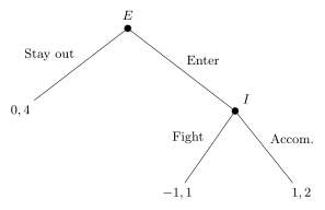
The pathology is sharpest in the chain-store game (Figure 3.5). A potential entrant chooses to stay out, ending the game at \((0,4)\), or to enter, after which the incumbent monopolist chooses to fight a price war, paying \((-1,1)\), or to accommodate, paying \((1,2)\). The normal-form representation has two Nash equilibria: \((\text{Enter}, \text{Accommodate})\) and \((\text{Stay out}, \text{Fight})\). The second is disturbing. It is sustained only by the incumbent’s threat to fight: anticipating a price war, the entrant stays out, so the threat is never tested. But the threat is not credible. If entry actually occurred, the incumbent compares fighting (\(1\)) with accommodating (\(2\)) and would strictly prefer to accommodate. The threat to fight is optimal only because, in equilibrium, the incumbent is never called upon to carry it out.
The remedy is to insist that each player behave optimally at every information set, on or off the path — that the player be sequentially rational. In a finite game of perfect information this is implemented by backward induction: start at the decision nodes whose successors are all terminal, fix each such player’s optimal action there, fold those payoffs back up the tree, and repeat, working from the leaves toward the root. The actions retained constitute a backward-induction solution.
In the chain-store game, backward induction first resolves the incumbent’s node — accommodate, since \(2 > 1\) — and then the entrant’s, who, foreseeing accommodation, enters since \(1 > 0\). The unique backward-induction solution is \((\text{Enter}, \text{Accommodate})\), and the non-credible equilibrium is discarded. Applying the same procedure to the sequential Battle of the Sexes (Figure 3.2): player \(2\) plays \(o\) after \(O\) (since \(1 > 0\)) and \(f\) after \(F\) (since \(2 > 0\)), giving the plan \(of\); player \(1\), foreseeing this, chooses \(O\) (since \(2 > 1\)). The unique backward-induction solution is \((O, of)\) — one of the three Nash equilibria, while the other two, \((O, oo)\) and \((F, ff)\), are eliminated.
A more dramatic illustration is the centipede game (Figure 3.6). Players alternate; at each of four successive decision nodes the mover can continue (passing a growing pie across the table) or stop and take the current split. Continuing to the very end yields \((3,3)\), while the stopping payoffs are, in order, \(1\)’s first stop \((1,1)\), \(2\)’s first stop \((0,3)\), \(1\)’s second stop \((2,2)\) and \(2\)’s second stop \((1,4)\).
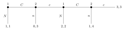
Writing a player’s strategy as her actions at her two nodes, the normal-form representation is
| \(nn\) | \(nc\) | \(cn\) | \(cc\) | |
|---|---|---|---|---|
| \(NN\) | \(1,\,1\) | \(1,\,1\) | \(1,\,1\) | \(1,\,1\) |
| \(NC\) | \(1,\,1\) | \(1,\,1\) | \(1,\,1\) | \(1,\,1\) |
| \(CN\) | \(0,\,3\) | \(0,\,3\) | \(2,\,2\) | \(2,\,2\) |
| \(CC\) | \(0,\,3\) | \(0,\,3\) | \(1,\,4\) | \(3,\,3\) |
There are four pure Nash equilibria — \((NN, nn)\), \((NN, nc)\), \((NC, nn)\) and \((NC, nc)\) — all with the same outcome: player \(1\) stops immediately at \((1,1)\). Backward induction is stark. At the last node player \(2\) stops (\(4 > 3\)); foreseeing this, player \(1\) stops at her second node (\(2 > 1\)); foreseeing that, player \(2\) stops at his first node (\(3 > 2\)); foreseeing all of it, player \(1\) stops at the very first node (\(1 > 0\)). The unique backward-induction solution is \((NN, nn)\): cooperation unravels completely, and the players walk away with \((1,1)\) despite the available \((3,3)\).
Backward induction delivers exactly what we want, and three theorems record its standing. The first connects it back to Nash equilibrium.
Theorem 3.2 (Backward-induction solutions are Nash equilibria) Every backward-induction solution is a Nash equilibrium in pure strategies.
This is a consequence of the equivalence with subgame-perfect equilibrium established below (Theorem 3.5), via the chain \(\text{(@thm-3-oneshot)} \Rightarrow \text{(@thm-3-spe-bi)} \Rightarrow \text{(@thm-3-bi-ne)}\); the source states it without a standalone proof. The next two results, both due to Kuhn, settle existence and uniqueness.
Theorem 3.3 (Kuhn: existence of a backward-induction solution) Every finite game of perfect information has a backward-induction solution, and hence a pure-strategy Nash equilibrium.
Theorem 3.4 (Uniqueness of the backward-induction solution) Every finite game of perfect information has a unique backward-induction solution if no player is indifferent between any two terminal nodes.
Both are stated without proof; the procedure itself is constructive, which is the content of existence, and uniqueness follows because at each step the maximiser is unique exactly when the relevant payoffs are never tied. Theorem 3.3 has a striking corollary: chess, being a finite game of perfect information, has a backward-induction solution, so in principle it is “solved” — one of the players has a strategy guaranteeing at least a draw. That we cannot compute it reflects the size of the tree, not any gap in the theory.
Nash equilibrium asks only that strategies be mutually optimal given the equilibrium path. Off-path behaviour is unconstrained, so a player can profitably commit, on paper, to actions she would never actually take — the chain store’s threat to fight, player \(2\)’s threat to play \(f\) after \(O\) in the Battle of the Sexes. Sequential rationality closes the loophole by demanding optimal play at every information set, reached or not. Backward induction enforces it directly in finite perfect-information games; the next section generalises it to games with information sets.
3.5 Subgame-perfect equilibrium
Backward induction needs perfect information: with information sets we cannot in general “start at the bottom and fold up,” because a player may not know which of several nodes she is at. The generalisation replaces “node” with subgame — a self-contained portion of the tree that can be analysed in isolation — and requires the strategy profile to induce a Nash equilibrium in every subgame.
Definition 3.10 (Subgame) A (proper) subgame \(G\) of an extensive-form game \(\Gamma\) consists of a single non-terminal node together with all of its successors in \(\Gamma\), subject to the requirement that whenever a node \(x\) belongs to \(G\) and \(x'\) lies in the same information set as \(x\), then \(x'\) also belongs to \(G\). With its inherited information sets and payoffs, \(G\) is itself a game tree. A node \(x\) induces a subgame if and only if (i) \(x\) is a singleton information set, and (ii) whenever two nodes share an information set and one is a successor of \(x\), the other is too. The whole game \(\Gamma\) is itself a subgame; in a game of perfect information, every non-terminal node induces a subgame.
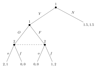
The closure condition is what keeps a subgame well-defined: we may not “cut into the middle” of an information set, because doing so would hand a player information — namely, which part of the set she is in — that the original game denied her. In the voluntary Battle of the Sexes below (Figure 3.7), the node where player \(1\) chooses \(Y\) versus \(N\) induces a subgame (the whole game), and the node where she then chooses \(O\) versus \(F\) induces a subgame (the embedded simultaneous game); but neither of player \(2\)’s nodes induces a subgame, because they share an information set, so cutting at one would separate it from its partner.
Definition 3.11 (Subgame-perfect equilibrium) A behavioral strategy profile \(\sigma^* = (\sigma_1^*, \dots, \sigma_n^*)\) is a subgame-perfect equilibrium (SPE) if, for every subgame \(G\) of \(\Gamma\), the restriction of \(\sigma^*\) to \(G\) is a Nash equilibrium of \(G\). “Every subgame” includes those reached and those not reached under \(\sigma^*\). In particular, since \(\Gamma\) is a subgame of itself, every SPE is a Nash equilibrium.
SPE is the refinement we sought: it demands mutual best responses both on and off the equilibrium path. In the chain-store game it strips out \((\text{Stay out}, \text{Fight})\), because the subgame following entry is the incumbent’s choice, and in that subgame “fight” is not a Nash equilibrium (accommodating pays more). Only \((\text{Enter}, \text{Accommodate})\) survives. For finite perfect-information games the new concept reduces to the old.
Theorem 3.5 (SPE equals backward induction in finite perfect-information games) For finite games of perfect information, the set of pure-strategy subgame-perfect equilibria coincides with the set of backward-induction solutions.
Proof. In a perfect-information game every non-terminal node induces a subgame, so SPE requires the strategy to be a Nash equilibrium starting from every node. Backward induction requires, at each node, that the prescribed action be optimal given the (already fixed) future play of all players. These are the same requirement node by node, so an SPE must be a backward-induction solution. The converse — that a backward-induction solution is an SPE — is delivered by the one-shot deviation principle (Theorem 3.6) below. \(\square\)
Verifying that a profile is an SPE could in principle require checking, in every subgame, that no player wants to switch to any alternative continuation strategy — a daunting task in a large tree. The one-shot deviation principle reduces this to checking only the simplest possible deviations: changing the prescribed action at a single information set and conforming everywhere else.
Definition 3.12 (One-shot deviation) A strategy \(s_i'\) is a one-shot deviation from \(s_i\) if it differs from \(s_i\) at one and only one information set: there is a unique \(h_i \in H_i\) with \(s_i'(h_i) \ne s_i(h_i)\), while \(s_i'(h_i') = s_i(h_i')\) for every \(h_i' \ne h_i\). (Also called a one-step or one-stage deviation.)
Definition 3.13 (Profitable one-shot deviation) Given a profile \(s\), a strategy \(s_i'\) is a profitable one-shot deviation if (i) \(s_i'\) is a one-shot deviation from \(s_i\) at some information set \(h_i\), and (ii) \(s_i'\) is a profitable deviation from \(s_i\) in the subgame induced by \(h_i\), given the opponents’ strategies \(s_{-i}\).
Theorem 3.6 (One-shot deviation principle) Consider a finite game of perfect information. A profile \(s\) is a subgame-perfect equilibrium if and only if no player has a profitable one-shot deviation.
The principle is stated without a formal proof; the source records the implication chain \(\text{(@thm-3-oneshot)} \Rightarrow \text{(@thm-3-spe-bi)} \Rightarrow \text{(@thm-3-bi-ne)}\), and notes that variants of the principle hold in all the games studied in this course. The intuition is a telescoping argument: if no single-step change helps anywhere in the tree, then no finite combination of changes can help either, because any multi-step deviation can be decomposed into one-shot pieces, none of which improves the payoff. This is what makes SPE checkable in practice — one need only confirm, at each node, that the prescribed action beats every immediate alternative, holding fixed all future play.
3.6 Subgame-perfect equilibrium: examples
The voluntary Battle of the Sexes
Return to the game of Figure 3.7, in which player \(1\) first chooses whether to play (\(Y\)) the Battle of the Sexes or take an outside option (\(N\)) worth \((1.5, 1.5)\); after \(Y\), the two play the simultaneous Battle of the Sexes \((O,o)=(2,1)\), \((O,f)=(0,0)\), \((F,o)=(0,0)\), \((F,f)=(1,2)\). Player \(1\)’s strategy specifies both the \(Y/N\) choice and the action in the subgame, so \(S_1 = \{YO, YF, NO, NF\}\) (e.g. \(NF\) = “opt out, but play \(F\) if the subgame were reached”); player \(2\) chooses \(o\) or \(f\). The normal form is
| \(o\) | \(f\) | |
|---|---|---|
| \(YO\) | \(2,\,1\) | \(0,\,0\) |
| \(YF\) | \(0,\,0\) | \(1,\,2\) |
| \(NO\) | \(1.5,\,1.5\) | \(1.5,\,1.5\) |
| \(NF\) | \(1.5,\,1.5\) | \(1.5,\,1.5\) |
Checking best responses gives three pure-strategy Nash equilibria: \((YO, o)\), \((NO, f)\) and \((NF, f)\). But not all are subgame perfect. The only proper subgame is the simultaneous Battle of the Sexes reached after \(Y\), whose Nash equilibria are the two pure profiles \((O,o)\) and \((F,f)\) and the mixed profile \(\big(\tfrac23 O + \tfrac13 F,\ \tfrac13 o + \tfrac23 f\big)\). Subgame perfection demands that the continuation play be one of these:
- If the subgame plays \((O,o)\), player \(1\) earns \(2 > 1.5\), so she plays \(Y\): the SPE is \((YO, o)\).
- If the subgame plays \((F,f)\), player \(1\) earns \(1 < 1.5\), so she opts out: the SPE is \((NF, f)\).
- The Nash equilibrium \((NO, f)\) is not subgame perfect: its continuation \((O, f)\) is not a Nash equilibrium of the subgame (given \(f\), player \(1\) would switch to \(F\)), so it rests on behaviour that is not sequentially rational off the equilibrium path.
There is also a mixed-strategy SPE: play the mixed equilibrium \(\big(\tfrac23 O + \tfrac13 F,\ \tfrac13 o + \tfrac23 f\big)\) in the subgame, which yields player \(1\) only \(\tfrac23 < 1.5\), so again she opts out. This is the dynamic counterpart of the mixed equilibrium from Chapter 2, now embedded as off-path continuation play. The example shows two things at once: subgame perfection genuinely refines Nash equilibrium (it discards \((NO,f)\)), and a single game can have several subgame-perfect equilibria, pure and mixed.
Stackelberg competition
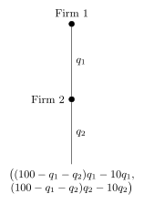
The Cournot duopoly of Chapter 2 had firms choose quantities simultaneously. Stackelberg competition makes the moves sequential: firm \(1\) (the leader) commits to a quantity \(q_1 \ge 0\), firm \(2\) (the follower) observes it and then chooses \(q_2 \ge 0\). Inverse demand is \(P = 100 - Q\) with \(Q = q_1 + q_2\), and each firm has constant marginal cost \(10\), so profits are \[ \pi_i(q_1, q_2) = (100 - q_1 - q_2)\,q_i - 10\,q_i . \] This is an (infinite) game of perfect information: firm \(1\)’s strategy is a number \(q_1 \in \R_+\), while firm \(2\)’s strategy is a function \(q_2(\cdot) : \R_+ \to \R_+\) specifying a response to each possible leader quantity. We solve it by backward induction.
In the subgame following any \(q_1\), the follower solves \(\max_{q_2 \ge 0} (100 - q_1 - q_2)\,q_2 - 10\,q_2\). The first-order condition \(90 - q_1 - 2 q_2 = 0\) gives the follower’s best response \[ q_2^*(q_1) = \frac{90 - q_1}{2} \qquad (\text{for } q_1 \le 90). \] Anticipating this, the leader solves \[ \max_{q_1 \ge 0}\ \Big(100 - q_1 - \tfrac{90 - q_1}{2}\Big)\,q_1 - 10\,q_1 . \] The first-order condition yields \(q_1^* = 45\), and then \(q_2^*(q_1^*) = \tfrac{90 - 45}{2} = 22.5\). The resulting profits are \[ \pi_1^* = 1012.5, \qquad \pi_2^* = 506.25 . \] Compare the simultaneous Cournot outcome, \(q_1^* = q_2^* = 30\) with \(\pi_1^* = \pi_2^* = 900\). The leader produces more and earns more, the follower less: there is a first-mover advantage. The source of the advantage is commitment. By moving first and visibly locking in a large quantity, the leader forces the follower to scale back, something a simultaneous mover could not credibly do.
We may sketch the tree schematically (Figure 3.8): each player has a continuum of branches, drawn as a single representative edge labelled by the chosen quantity.
It is worth noting that, as in the chain-store game, the extensive game has many Nash equilibria that are not subgame-perfect. Fix any \(\hat q_1 \ge 0\) with \((100 - \hat q_1 - q_2^*(\hat q_1))\,\hat q_1 - 10\,\hat q_1 \ge 0\), and let firm \(2\) adopt the rule “play \(q_2^*(\hat q_1)\) if \(q_1 = \hat q_1\), and flood the market with \(q_2 = 90\) otherwise.” Against this rule the leader’s best choice is \(\hat q_1\), so \((\hat q_1, \hat q_2(\cdot))\) is a Nash equilibrium. But the threat to set \(q_2 = 90\) — which drives the price down to \(10\), exactly marginal cost, wiping out all margin — is not credible: off the path it is not a best response, so the profile is not an SPE. Subgame perfection again selects the sensible outcome.
Mutually assured destruction
The Cuban missile crisis of \(1962\) can be stylised as a game of escalation between the United States (player \(1\)) and the Soviet Union (player \(2\)); see Figure 3.9. Player \(1\) first chooses to ignore (\(I\)) the Soviet missiles, ending the game at \((0,0)\), or to escalate (\(E\)). After \(E\), player \(2\) chooses to back down (\(B\)), paying \((10, -10)\), or to go nuclear (\(N\)). After \(N\) the two superpowers play a simultaneous brinkmanship subgame: each may retreat (\(R\) for player \(1\), \(r\) for player \(2\)) or trigger doomsday (\(D\), \(d\)). If both retreat the payoff is \((-5,-5)\); if either chooses doomsday the payoff is the catastrophe \((-100, -100)\).
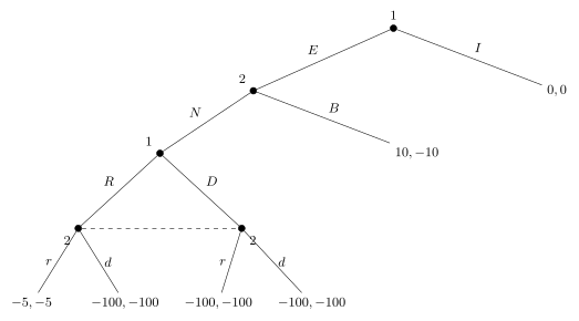
The inner simultaneous subgame has the bimatrix
| \(r\) | \(d\) | |
|---|---|---|
| \(R\) | \(-5,\,-5\) | \(-100,\,-100\) |
| \(D\) | \(-100,\,-100\) | \(-100,\,-100\) |
This subgame has two pure Nash equilibria, and each generates a distinct SPE of the whole game.
- If the subgame plays \((R, r)\), paying \((-5,-5)\): working backward, after \(E\) player \(2\) prefers \(N\) (giving \(-5\)) to \(B\) (giving \(-10\)); and at the root player \(1\) prefers \(I\) (giving \(0\)) to \(E\) (giving \(-5\)). The resulting SPE is \((IR,\ Nr)\) — player \(1\) plays \(I\), then \(R\); player \(2\) plays \(N\), then \(r\).
- If the subgame plays \((D, d)\), paying \((-100,-100)\): after \(E\) player \(2\) now prefers \(B\) (giving \(-10\)) to \(N\) (giving \(-100\)); and at the root player \(1\) prefers \(E\) (giving \(10\)) to \(I\) (giving \(0\)). The resulting SPE is \((ED,\ Bd)\) — player \(1\) plays \(E\), then \(D\); player \(2\) plays \(B\), then \(d\).
So there are two pure-strategy subgame-perfect equilibria, \((IR, Nr)\) and \((ED, Bd)\), corresponding to the two equilibria of the brinkmanship subgame. The multiplicity is the substantive point: which equilibrium prevails depends on what each side believes the other would do at the brink, and a credible commitment to doomsday (\(D, d\)) — however terrifying — deters escalation and yields the more peaceful path \((ED, Bd)\), in which player \(1\) escalates and player \(2\) backs down. This is the logic of deterrence by mutually assured destruction.
3.7 Repeated games
Many of the most interesting strategic situations are not one-shot encounters but ongoing relationships: firms that compete in the same market quarter after quarter, neighbours who trade favours, countries that bargain repeatedly. The basic question is whether the shadow of the future can sustain cooperation that is impossible in a single play. Repeated games give the formal answer.
Fix a normal-form game \(G = (N, \{A_i\}, \{v_i\})\) — the stage game — and play it \(T\) times, where \(T\) is either a finite number or \(T = \infty\). In each period \(t\) the players choose an action profile \(a^t = (a_1^t, \dots, a_n^t) \in A\), where \(A = A_1 \times \cdots \times A_n\) is the set of stage action profiles, and \(v_i(a^t)\) is \(i\)’s stage payoff in period \(t\). Crucially, the players observe the entire past before moving: the game is one of perfect information at the level of action profiles, even when the stage game itself has simultaneous moves.
Discounting. Players value a euro today more than a euro tomorrow, so future stage payoffs are weighted by a discount factor \(\delta\). For a finitely repeated game \(\delta \in (0,1]\); for an infinitely repeated game \(\delta \in (0,1)\) (so that the infinite sum converges). Player \(i\)’s payoff for the whole repeated game is the discounted sum of stage payoffs, \[ v_i = \sum_{t=1}^{T} \delta^{t-1}\, v_i^{t}, \] where \(v_i^t = v_i(a^t)\). In the infinite-horizon case it is conventional to use the average discounted payoff, which simply rescales by \((1-\delta)\): \[ v_i \;\equiv\; (1-\delta) \sum_{t=1}^{\infty} \delta^{t-1}\, v_i^{t}. \] The normalisation is convenient because if a fixed profile \(a\) is played in every period, then \((1-\delta)\sum_{t\ge1}\delta^{t-1} v_i(a) = v_i(a)\): the average discounted payoff of “always \(a\)” is just the one-period payoff \(v_i(a)\), so repeated-game payoffs live on the same scale as stage payoffs.
Histories and strategies. What a player can condition on is the record of what has happened. A history at the start of period \(t\) is the list of past action profiles \(h_t = (a^1, \dots, a^t) \in A^t =: H_t\), with the empty history \(H_0 = \{\varnothing\}\) describing the initial node. A (pure) strategy for player \(i\) is a map from histories to actions, \[ s_i : \bigcup_{t=0}^{T-1} H_t \to A_i , \] equivalently a list \((s_i^1, s_i^2, \dots)\) with \(s_i^t : H_{t-1} \to A_i\) telling \(i\) what to play in period \(t\) as a function of everything observed so far. A strategy is therefore a complete contingent plan, and the solution concept we carry over is subgame-perfect equilibrium (Definition 3.11): the profile must induce a Nash equilibrium in every subgame, i.e. after every history.
Finitely repeated games
When the horizon is finite, backward induction starts from the last period. There the future is empty, so each player simply plays the stage game — and an SPE must therefore prescribe a stage Nash equilibrium at the end.
Lemma 3.1 (last-period play). Suppose \(s\) is an SPE of a finitely repeated game. In the last period, after any history, \(s\) must play a stage Nash equilibrium. (After different histories, different stage equilibria may be played.)
This is the engine of the next theorem, which records two facts: repeating any single stage equilibrium is always an SPE, and if the stage game has a unique Nash equilibrium then that repetition is the only SPE — so a finite horizon buys no extra cooperation when the stage game is “solved”.
Theorem 3.7 (Repetition of a stage equilibrium) Consider a finitely repeated game. If \(a^* = (a_1^*, \dots, a_n^*)\) is a Nash equilibrium of the stage game, then the profile \(s\) that plays \(a^*\) after every history is an SPE of the repeated game, for any \(\delta \in (0,1]\). If, in addition, \(a^*\) is the unique stage Nash equilibrium, then this profile is the unique SPE.
Proof. Part 1: \(s\) is an SPE. We verify directly. Consider any history \(h = (\tilde a^1, \dots, \tilde a^{t-1})\) reached at the start of period \(t \in \{1, \dots, T\}\). In the subgame following \(h\), holding the opponents’ strategies fixed at “always \(a_{-i}^*\)”, player \(i\)’s payoff from any strategy is \[ \sum_{\tau=1}^{t-1} \delta^{\tau-1} v_i(\tilde a^\tau) \;+\; \sum_{\tau=t}^{T} \delta^{\tau-1} v_i(a_i^\tau, a_{-i}^*). \] The first sum is sunk. Because \(a_i^*\) maximises \(i\)’s stage payoff when the opponents play \(a_{-i}^*\), choosing \(a_i^\tau = a_i^*\) in every remaining period maximises each term of the second sum. Hence playing \(s_i\) is optimal in this subgame, and \(s\) is an SPE.
Part 2: uniqueness when \(a^*\) is unique. Take any SPE \(\tilde s\) and consider a history \(h = (\tilde a^1, \dots, \tilde a^{T-1})\) at the start of the last period. The subgame is a simultaneous-move game with strategy spaces \(A_i\) and payoffs \[ \hat v_i(a) = \sum_{\tau=1}^{T-1} \delta^{\tau-1} v_i(\tilde a^\tau) \;+\; \delta^{T-1} v_i(a), \] which differs from the stage game only by the sunk constant and a positive scale \(\delta^{T-1}\); the two are strategically equivalent. Since \(\tilde s\) is an SPE it plays a Nash equilibrium here, which must be the unique stage equilibrium: \(\tilde s_i^T(h) = a_i^*\) for all \(i\) and all \(h \in H_{T-1}\).
Induction step. Suppose \(\tilde s\) plays \(a^*\) in every period \(t = k, k+1, \dots, T\) after every history; we show the same for period \(t = k-1\). Fix any history \(h = (\tilde a^1, \dots, \tilde a^{t-1}) \in H_{t-1}\). Because \(\tilde s\) is an SPE there is no profitable deviation after \(h\), so each \(\tilde s_i^t(h)\) solves \[ \max_{a_i \in A_i}\; \sum_{\tau=1}^{t-1} \delta^{\tau-1} v_i(\tilde a^\tau) \;+\; \delta^{t-1} v_i(a_i, \tilde s_{-i}^t(h)) \;+\; \sum_{\tau=t+1}^{T} \delta^{\tau-1} v_i(a^*). \] The first and last sums do not depend on \(a_i\), so this is equivalent to \(\max_{a_i} v_i(a_i, \tilde s_{-i}^t(h))\). Thus \(\tilde s^t(h)\) is a stage Nash equilibrium and equals \(a^*\) by uniqueness. By induction \(\tilde s\) plays \(a^*\) after every history, so it is the profile \(s\). \(\square\)
So repetition by itself is powerless against a uniquely-solved stage game such as the Prisoner’s Dilemma: with a finite horizon the only SPE is to defect every period.
Cooperation through multiple stage equilibria. The picture changes once the stage game has more than one Nash equilibrium, because then the players can use the choice among them as a system of rewards and punishments. Consider the augmented partnership game, in which each player can put in effort (\(E\)), shirk (\(S\)), or take a mutually destructive punishment action (\(P\)):
| \(E\) | \(S\) | \(P\) | |
|---|---|---|---|
| \(E\) | \(2,\,2\) | \(-1,\,3\) | \(-3,\,-3\) |
| \(S\) | \(3,\,-1\) | \(0,\,0\) | \(-3,\,-3\) |
| \(P\) | \(-3,\,-3\) | \(-3,\,-3\) | \(-2,\,-2\) |
This game has two pure stage Nash equilibria, \(SS\) (payoff \(0,0\)) and \(PP\) (payoff \(-2,-2\)); the cooperative profile \(EE\) (payoff \(2,2\)) is not an equilibrium, since each player would deviate to \(S\). By Theorem 3.7 applied to the last period, \(EE\) can never be played in the final period after any history. But over two periods cooperation can arise in the first period, sustained by a carrot-and-stick continuation: \[ s_i^1 = E, \qquad s_i^2(h) = \begin{cases} S & \text{if } h = EE, \\ P & \text{if } h \ne EE. \end{cases} \] The carrot is the good equilibrium \(SS\) (payoff \(0\)) played as a reward for cooperation; the stick is the bad equilibrium \(PP\) (payoff \(-2 < 0\)) triggered by any first-period deviation. Both continuations are stage equilibria, so the second period is incentive-compatible regardless. The only question is whether \(E\) beats a first-period deviation. Comparing player 1’s options, given the prescribed continuation:
- Play \(E\): \(v_1(EE) + \delta\, v_1(SS) = 2 + \delta\cdot 0 = 2\).
- Deviate to \(S\): \(v_1(SE) + \delta\, v_1(PP) = 3 + \delta\cdot(-2) = 3 - 2\delta\).
- Deviate to \(P\): \(v_1(PE) + \delta\, v_1(PP) = -3 - 2\delta\).
The action \(E\) is optimal iff \(2 \ge 3 - 2\delta\), i.e. \(\delta \ge \tfrac12\) (the \(P\) deviation is never tempting). By symmetry the same holds for player 2.
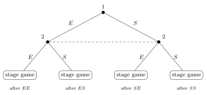
For \(\delta \ge \tfrac12\), the profile above is an SPE with cooperation \(EE\) on the equilibrium path of the first period. Patience matters: only when the future weighs at least half as much as the present is the one-period gain from cheating (\(3\) vs \(2\)) outweighed by the loss of switching from the carrot \(SS\) to the stick \(PP\). The twice-repeated unaugmented partnership game (Figure 3.10) has no such room — its stage game has the unique equilibrium \(SS\), so by Theorem 3.7 its only SPE plays \(S\) after every history, with outcome path \((SS, SS)\) for every \(\delta\).
Infinitely repeated games
With an infinite horizon there is no last period to anchor backward induction, but the structure is in some ways simpler: every subgame looks exactly like the whole game. Indeed, after any history \(h\) of length \(t\) the continuation game is itself an infinitely repeated \(G\), and the continuation payoff differs from a fresh start’s only by the discount factor \(\delta^{t}\). This self-similarity gives a clean characterisation.
Lemma 3.2 (SPE characterisation). Consider a profile \(s\) in an infinitely repeated game. Then \(s\) is an SPE if and only if the continuation play of \(s\) after any history \(h\) is itself a Nash equilibrium of the original repeated game.
The justification is exactly the self-similarity just described: a subgame of an infinitely repeated game is equivalent (up to a \(\delta^{t}\) factor) to the whole repeated game, so “Nash in every subgame” reduces to “every continuation is Nash in the repeated game”. With this in hand, the analogue of the finite-horizon repetition result is immediate.
Theorem 3.8 (Repetition of a stage equilibrium, infinite horizon) Consider an infinitely repeated game. If \(a = (a_1, \dots, a_n)\) is a stage Nash equilibrium, then the profile \(s\) that plays \(a\) after every history is an SPE, for any \(\delta \in (0,1)\).
Proof. By Lemma 3.2 it suffices to show that \(s\) is a Nash equilibrium of the repeated game. Given \(s_{-i}\) (which always plays \(a_{-i}\)), always playing \(a_i\) is optimal for \(i\), because \(a_i\) maximises \(i\)’s stage payoff against \(a_{-i}\) in every single period, hence maximises the discounted sum term by term. The argument does not depend on \(\delta\). \(\square\)
Grim trigger and the Prisoner’s Dilemma. Unlike the finite case, an infinite horizon can sustain cooperation even when the stage equilibrium is unique, because the threat of permanent reversion to the bad equilibrium never runs out of periods. The canonical device is the grim-trigger strategy: cooperate as long as everyone has always cooperated, and switch forever to the stage equilibrium the instant anyone deviates. In the partnership game (stage payoffs as in Table 3.5 restricted to \(\{E,S\}\), with unique equilibrium \(SS\)), grim trigger is \[ s_i^t(h) = \begin{cases} E & \text{if } h = \varnothing \text{ or } h = (EE, \dots, EE) \in H_{t-1}, \\ S & \text{otherwise.} \end{cases} \] Using average discounted payoffs, compare player \(i\)’s options at the empty history:
- Cooperate (\(E\) forever along the path): \(v_i(EE) = 2\).
- Deviate once to \(S\), triggering \(SS\) forever after: \((1-\delta) v_i(SE) + \delta\, v_i(SS) = (1-\delta)\cdot 3 + \delta\cdot 0 = 3(1-\delta)\).
There is no profitable one-shot deviation iff \(2 \ge 3(1-\delta)\), i.e. \(\delta \ge \tfrac13\). After any history of the form \((EE,\dots,EE)\) the continuation is \(s\) itself, giving the same condition; after any history containing an \(S\), the continuation simply repeats the stage equilibrium \(SS\), which is an SPE by Theorem 3.8 for every \(\delta\). Hence grim trigger is an SPE iff \(\delta \ge \tfrac13\), sustaining cooperation \(EE\) forever.
The same logic delivers a general sustainability theorem: any action profile that strictly Pareto-improves on a stage equilibrium can be supported in an SPE once players are patient enough.
Theorem 3.9 (Sustaining a cooperative path) Consider an infinitely repeated game. Suppose \(a^* = (a_1^*, \dots, a_n^*)\) is a stage Nash equilibrium, and there is an action profile \(a = (a_1, \dots, a_n)\) giving every player a strictly higher stage payoff than \(a^*\). Then there exists \(\bar\delta \in (0,1)\) such that for every \(\delta \ge \bar\delta\) there is an SPE whose outcome path is the repeated play of \(a\).
Proof. Let \(M \equiv \max_{i,\,a'} v_i(a')\) be the largest stage payoff over all players and all action profiles, and consider the trigger profile \[ s_i^t(h) = \begin{cases} a_i & \text{if } h = \varnothing \text{ or } h = (a, \dots, a) \in H_{t-1}, \\ a_i^* & \text{otherwise,} \end{cases} \qquad t \ge 1. \] We check for profitable one-shot deviations after every history.
Period 1. If \(i\) plays \(a_i\), the average discounted payoff is \(v_i(a)\). If \(i\) deviates to some \(a_i' \ne a_i\), then (since the deviation triggers reversion to \(a^*\) forever) the payoff is \[ (1-\delta) v_i(a_i', a_{-i}) + \delta\, v_i(a^*) \;\le\; (1-\delta) M + \delta\, v_i(a^*). \] There is no profitable one-shot deviation in period 1 provided \(v_i(a) \ge (1-\delta) M + \delta\, v_i(a^*)\), which rearranges to \[ \delta \ge \delta_i \equiv \frac{M - v_i(a)}{M - v_i(a^*)} \in [0,1), \] the membership in \([0,1)\) holding because \(v_i(a) > v_i(a^*)\). Set \(\bar\delta \equiv \max_i \delta_i\). Then for \(\delta \in [\bar\delta, 1)\) no player has a profitable one-shot deviation in period 1.
History \(h = (a, \dots, a)\). The continuation play is exactly \(s\) again, so the period-1 argument applies verbatim: no profitable one-shot deviation for \(\delta \in [\bar\delta, 1)\).
History \(h \ne (a, \dots, a)\). The continuation play is the repeated play of the stage equilibrium \(a^*\) after every further history, which is an SPE of the subgame by Theorem 3.8; hence no profitable one-shot deviation, for any \(\delta\).
So for \(\delta \in [\bar\delta, 1)\) there is no profitable one-shot deviation after any history, and by the one-shot deviation principle (Theorem 3.6) the profile is an SPE. \(\square\)
Cournot collusion. A celebrated application is tacit collusion among Cournot competitors. Take the duopoly with inverse demand \(P(Q) = \max\{100 - Q,\, 0\}\), \(Q = q_1 + q_2\), and constant marginal cost \(c_1 = c_2 = 10\), played each period with discount \(\delta \in (0,1)\). Two benchmarks frame the analysis:
- Collusion (monopoly split). Maximising joint profit \(\max_Q [P(Q) - 10]Q\) gives the monopoly quantity \(Q^* = 45\); splitting it equally, each firm produces \(q^c = 22.5\) and earns \(45 \times 22.5 = 1012.5\) per period.
- Stage Nash equilibrium (Cournot). The static equilibrium is \(q^e = 30\) for each firm, earning \(30 \times 30 = 900\) per period.
Consider the trigger profile: produce the collusive \(q_i^c\) as long as both firms have always done so, and revert forever to the Cournot \(q_i^e\) otherwise. By Theorem 3.8 the reversion phase is an SPE; the binding constraint is again the first period. The most tempting one-shot deviation is the static best response to the partner’s \(q^c = 22.5\), namely \(q_i = (90 - 22.5)/2 = 33.75\), which yields the one-period profit \[ (100 - 33.75 - 22.5 - 10)\cdot 33.75 = 33.75 \times 33.75 = 1139.0625 . \] There is no profitable deviation iff staying collusive beats deviating-then-being- punished, in average discounted terms: \[ 1012.5 \;\ge\; (1-\delta)\cdot 1139.0625 + \delta\cdot 900 . \] Rearranging, \(1012.5 - 900 = (1-\delta)(1139.0625 - 900)\), i.e. \(112.5 = (1-\delta)\cdot 239.0625\), so \(1 - \delta = 0.4706\ldots\) and \[ \delta \;\ge\; \bar\delta \approx 0.5294 , \] which the slides round to \(\delta \ge 0.53\). For \(\delta\) above this threshold the collusive trigger profile is an SPE, and the firms sustain the monopoly outcome period after period — collusion that the law forbids but that patient repetition makes self-enforcing.
3.8 Strategic bargaining
How is a fixed surplus divided when the parties can make and reject offers over time? The alternating-offer model gives a sharp, dynamic answer. A pie of size \(1\) is to be split; the players alternate making proposals, with player 1 proposing in odd rounds and player 2 in even rounds, and the proposer’s share is listed first. A proposal \((x, 1-x)\) with \(x \in [0,1]\) is either accepted — ending the game — or rejected, in which case play passes to the next round. Delay is costly: agreement on \((x, 1-x)\) reached in round \(t\) is worth \(\delta^{t-1} x\) to player 1 and \(\delta^{t-1}(1-x)\) to player 2, with discount \(\delta \in (0,1)\). This is a game of perfect information, so we solve it by backward induction.
\(T = 1\): the ultimatum game. With a single round, player 1 makes a take-it-or-leave-it offer; rejection destroys the pie, leaving both with \(0\). For any \(x < 1\), player 2 strictly prefers to accept (getting \(1 - x > 0\)); at \(x = 1\) she is indifferent. The unique SPE has player 1 propose \((1, 0)\) and player 2 accept every proposal — including the knife-edge \((1,0)\), since the alternative of accepting all offers except \((1,0)\) leaves player 1 with no best response (he would want to offer the largest \(x < 1\), which does not exist). The unique SPE outcome is \((1, 0)\): the proposer takes the entire pie. Many other Nash equilibria exist (e.g. player 2 threatens to accept only one specific offer), but they rest on incredible threats.
\(T = 2\). Now if player 2 rejects the round-1 offer, she becomes the proposer in round 2 and — facing the deadline — can claim the whole (discounted) pie, worth \(\delta\) to her. So in round 1 she accepts \((x, 1-x)\) iff \(1 - x \ge \delta\) (accepting when indifferent, again because otherwise player 1 has no optimum). Player 1 therefore offers the smallest share that secures acceptance, \(1 - x = \delta\), proposing \((1-\delta, \delta)\). This is the unique SPE: agreement is immediate, with equilibrium payoff \((1-\delta, \delta)\). The threat of becoming next period’s dictator hands player 2 a share \(\delta\), which grows toward \(\tfrac12\) as \(\delta \to 1\).
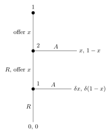
\(T = 3\). If round 1 is rejected, the remaining two rounds are exactly the \(T=2\) game with the roles swapped and one period of discounting applied, giving continuation payoffs \((\delta^2,\, \delta(1-\delta))\). Player 2’s round-1 continuation value is thus \(\delta(1-\delta)\), so she accepts any \((x,1-x)\) with \(1 - x \ge \delta(1-\delta)\), and player 1 proposes \[ \big(\, 1 - \delta(1-\delta),\; \delta(1-\delta) \,\big). \]
\(T = 4\). One more layer of backward induction nests the discount once more, and player 1 proposes \[ \big(\, 1 - \delta\big(1 - \delta(1-\delta)\big),\; \delta\big(1 - \delta(1-\delta)\big) \,\big). \] The pattern is a nested, alternating-sign geometric series — each extra round of horizon adds another term \(\pm\delta^{k}\) — and longer finite deadlines continue analogously.
Rubinstein’s infinite-horizon model. Letting \(T = \infty\) removes the deadline and, remarkably, restores a unique prediction. The game is stationary: every subgame in which player 1 proposes looks identical, as does every subgame in which player 2 proposes. This suggests a stationary SPE in which player 1 always offers \((x^*, 1-x^*)\), player 2 always offers \((y^*, 1-y^*)\) (player 1’s share listed first, so player 2 keeps \(1-y^*\)), and each accepts exactly when offered at least their stationary continuation value. For the proposer’s offer to be optimal, the responder must be made just indifferent between accepting now and rejecting to become tomorrow’s proposer:
- Player 2 is indifferent at her offered share \(1 - x^*\): \(1 - x^* = \delta(1 - y^*)\).
- Player 1 is indifferent at his offered share \(y^*\): \(y^* = \delta x^*\).
Substituting \(y^* = \delta x^*\) into the first equation gives \(1 - x^* = \delta - \delta^2 x^*\), hence \(1 - \delta = x^*(1 - \delta^2)\) and \[ x^* = \frac{1-\delta}{1-\delta^2} = \frac{1}{1+\delta}, \qquad y^* = \frac{\delta}{1+\delta}. \tag{3.1}\] Agreement is immediate and the first proposer, player 1, secures \(x^* = 1/(1+\delta)\). As \(\delta \to 1\) the split approaches \((\tfrac12, \tfrac12)\): when players are patient, the first-mover advantage vanishes.
The truly striking fact is that this stationary equilibrium is the unique SPE.
Let \(G_i\) be the set of all SPE payoffs to player \(i\) across subgames in which player \(i\) proposes first, and write \(M_i = \sup G_i\), \(m_i = \inf G_i\). We bound these four numbers and squeeze them to a point.
Claim A: \(m_i \ge 1 - \delta M_j\) for \(i \ne j\). Take \(i=1\), \(j=2\). In a subgame where player 1 proposes, if player 2 rejects she becomes the proposer in a subgame worth at most \(\delta M_2\) to her. So she accepts any offer giving her strictly more than \(\delta M_2\), which lets player 1 secure \(1 - \delta M_2 - \varepsilon\) for any \(\varepsilon > 0\). Hence \(m_1 \ge 1 - \delta M_2\).
Claim B: \(M_i \le 1 - \delta m_j\) for \(i \ne j\). Again \(i=1\), \(j=2\). If player 2 rejects, she gets at least \(\delta m_2\), so she rejects any offer giving her strictly less than \(\delta m_2\). If player 1’s offer is accepted he gets at most \(1 - \delta m_2\); if it is rejected he gets at most \(\delta(1 - m_2) \le 1 - \delta m_2\). Hence \(M_1 \le 1 - \delta m_2\).
Squeeze. Combining the two claims (and their symmetric counterparts), \[ m_i \ge 1 - \delta M_j \ge 1 - \delta(1 - \delta m_i) \;\Longrightarrow\; m_i \ge \tfrac{1}{1+\delta}, \] \[ M_i \le 1 - \delta m_j \le 1 - \delta(1 - \delta M_i) \;\Longrightarrow\; M_i \le \tfrac{1}{1+\delta}. \] Since \(m_i \le M_i\) always, both equal \(\tfrac{1}{1+\delta}\): the SPE payoff to the first proposer is uniquely \(1/(1+\delta)\), the stationary value.
Unique strategies. In any SPE where player 1 proposes, if no agreement is reached in round 1 then player 1 gets at most \(1 - M_2 = \delta M_1 < M_1\), so to attain \(M_1\) agreement must be immediate: player 1 offers \((M_1, 1-M_1)\) and player 2 accepts, rejecting anything that gives her strictly less than \(1 - M_1 = \delta M_2\) and accepting anything strictly more. The symmetric argument pins down player 2’s proposing subgames. Therefore the stationary SPE is the unique SPE. \(\square\)
A combinatorial cousin, the pirate game — \(n\) pirates dividing \(100\) coins by successive proposals, where a proposer is thrown overboard if at least half vote against him — is left as a bonus exercise; it is solved by the same backward reasoning, starting from the two-pirate endgame.
3.9 Chapter summary
- A repeated game plays a stage game \(G\) either \(T < \infty\) or \(\infty\) times; payoffs are the discounted sum \(\sum_t \delta^{t-1} v_i^t\), conventionally rescaled to the average discounted payoff \((1-\delta)\sum_t \delta^{t-1} v_i^t\) in the infinite case. Strategies map histories to actions, and the solution concept is SPE.
- Finitely repeated games: an SPE must play a stage equilibrium in the last period (Lemma 3.1); repeating any stage equilibrium is an SPE, and if the stage equilibrium is unique it is the only SPE (Theorem 3.7). Repetition alone buys no cooperation.
- With multiple stage equilibria (augmented partnership game), a carrot-and- stick continuation sustains cooperation \(EE\) in the first period when \(\delta \ge \tfrac12\).
- Infinitely repeated games: every subgame is equivalent to the whole game (Lemma 3.2), so continuation play must itself be a repeated-game equilibrium. Repeating a stage equilibrium is always an SPE (Theorem 3.8).
- Grim trigger sustains cooperation even with a unique stage equilibrium when players are patient: the Prisoner’s Dilemma cooperates for \(\delta \ge \tfrac13\). More generally, any strictly Pareto-improving profile is sustainable for \(\delta \ge \bar\delta\) (Theorem 3.9). Cournot collusion (\(q^c = 22.5\), profit \(1012.5\) versus Cournot \(q^e = 30\), profit \(900\)) is self-enforcing for \(\delta \ge \bar\delta \approx 0.5294\).
- Strategic bargaining: the ultimatum game (\(T=1\)) gives the proposer everything, \((1,0)\); finite alternating offers yield a nested geometric pattern (\(T=2\): \((1-\delta, \delta)\); \(T=3\): \((1-\delta(1-\delta), \delta(1-\delta))\)). Rubinstein’s infinite-horizon game has the unique SPE \(\big(\tfrac{1}{1+\delta}, \tfrac{\delta}{1+\delta}\big)\) (Equation 3.1), with immediate agreement; uniqueness follows from squeezing the sup/inf payoff bounds to \(M_i = m_i = 1/(1+\delta)\). As \(\delta \to 1\) the split tends to \((\tfrac12, \tfrac12)\).