8 Nonlinear Equations & Optimization

\[ \newcommand{\R}{\mathbb{R}} \newcommand{\C}{\mathbb{C}} \newcommand{\N}{\mathbb{N}} \newcommand{\E}{\mathbb{E}} \newcommand{\eps}{\varepsilon} \newcommand{\abs}[1]{\left\lvert #1 \right\rvert} \newcommand{\norm}[1]{\left\lVert #1 \right\rVert} \newcommand{\ninf}[1]{\left\lVert #1 \right\rVert_{\infty}} \newcommand{\ntwo}[1]{\left\lVert #1 \right\rVert_{2}} \newcommand{\none}[1]{\left\lVert #1 \right\rVert_{1}} \newcommand{\inner}[2]{\left\langle #1,\, #2 \right\rangle} \newcommand{\bigO}{\mathcal{O}} \newcommand{\dd}{\mathrm{d}} \newcommand{\diff}[2]{\frac{\mathrm{d} #1}{\mathrm{d} #2}} \newcommand{\pdiff}[2]{\frac{\partial #1}{\partial #2}} \newcommand{\spec}{\rho} \newcommand{\cond}{\kappa} \newcommand{\Span}{\operatorname{span}} \newcommand{\rank}{\operatorname{rank}} \newcommand{\tr}{\operatorname{tr}} \newcommand{\diag}{\operatorname{diag}} \newcommand{\argmax}{\operatorname*{arg\,max}} \newcommand{\argmin}{\operatorname*{arg\,min}} \newcommand{\defeq}{:=} \]

Solving an equation has, in every chapter so far, meant solving a linear one. Interpolation coefficients, spline curvatures, least-squares normal equations, and the systems of Chapter 4 and Chapter 5 are all instances of $Ax=b$, and for those we have finite, exact algorithms. The equations that come up in practice are usually not linear, and once we leave the linear world that comfort disappears: there is, in general, no formula that returns a root. The only general-purpose tool left is iteration: start from a guess, apply a rule that (we hope) improves it, and repeat until the sequence settles on a solution.

This chapter builds the two iterations that do most of the real work (fixed-point iteration and Newton’s method) and organizes them around one question rather than around the methods themselves: how fast does the error shrink from one step to the next? That rate is the order of convergence, and it splits our iterations cleanly into two tiers. Some methods peel off a fixed number of correct digits per step; we collect those in Section 8.2. Others accelerate, so that each step is cheaper than the last in digits per iteration; Newton’s method is the archetype, in Section 8.3.

One word needs pinning down before we start. “Order” here means order of convergence, how the error $\norm{x^{(k)}-x^\star}$ decays as the iteration count $k\to\infty$, and it is a different quantity from the order of accuracy $\bigO(h^p)$ of a discretization as a mesh size $h\to0$ (Chapter 2). The two share a word and nothing else, and the notes keep them apart (see Notation).

Two “orders”, one word

Both live in this book and neither is the other.

Order of accuracy $p$ (Chs. 2–3): a fixed rule applied at resolution $h$ commits error $\bigO(h^p)$; you improve it by refining the mesh, $h\to0$.
Order of convergence $q$ (this chapter): a single sequence of iterates has error obeying $\norm{x^{(k+1)}-x^\star}\le M\norm{x^{(k)}-x^\star}^{q}$; you improve it by taking more steps, $k\to\infty$.

Order of accuracy grades a discretization; order of convergence grades an iteration.

8.1 General nonlinear equations

The problem of the chapter is to solve a system of $n$ nonlinear equations in $n$ unknowns, \[ F(x)=0,\qquad F:\R^n\to\R^n . \tag{8.1}\] Stacking the scalar coordinate functions $f_i:\R^n\to\R$, \[ F(x)=\begin{pmatrix} f_1(x)\\ \vdots\\ f_n(x)\end{pmatrix}, \] turns Equation 8.1 into the simultaneous conditions $f_1(x)=\dots=f_n(x)=0$. The contrast with $Ax=b$ is sharp: a nonlinear system may have no solution, one, or many, and no direct method returns them. So we settle for iterative methods that, launched from an initial guess, home in on some solution, usually the one nearest the guess, when one exists.

Two families of problems account for most of what follows, and it is worth seeing them as special cases rather than as separate subjects. The first is linear systems themselves, $F(x)=Ax-b$, the entire content of Chapter 4 and Chapter 5. They are not a world apart from the nonlinear story: Newton’s method will attack a nonlinear $F$ by solving a fresh linear system $Ax=b$ at every step, so the LU machinery of Chapter 4 is a subroutine inside the nonlinear solver, not a competitor to it. The second is optimization: to find a critical point of a scalar objective $u:\R^n\to\R$ is to solve $\nabla u(x)=0$, i.e. to take $F=\nabla u$. The guarantees are strongest when $u$ is strictly convex (its Hessian $\nabla^2 u(x)=\bigl[\partial^2 u/\partial x_i\partial x_j\bigr]$ is positive definite everywhere) and that convex case, treated in Section 8.2.4, is where the condition-number story of Chapters 4–5 reappears.

The same equation Equation 8.1 also governs implicit time-stepping for stiff ODEs (Chapter 3) and discretized nonlinear PDEs, among much else; the two methods below serve all of these.

8.2 Linearly convergent iterations

Our first tier collects the iterations that converge linearly: the error is multiplied by a constant factor below $1$ at each step, so on a log scale it falls along a straight line. Every method here (fixed-point iteration, its Banach guarantee, the Jacobian test that makes the guarantee checkable, and gradient descent) is a single mechanism seen from different angles: an update map that contracts distances. In the language of Section 8.3.1, these are the $q=1$ methods, and their common weakness is that the contraction factor can sit uncomfortably close to $1$.

From roots to fixed points

Definition 8.1 (Fixed point) Given $g:\R^n\to\R^n$, a point $x$ is a fixed point of $g$ if $g(x)=x$.

Fixed-point iteration rewrites the root problem $F(x)=0$ as a fixed-point problem $g(x)=x$ with the same solution set, and then iterates the map $g$. Building such a $g$ takes no cleverness: pick any scalar $\eps\neq0$ and define \[ g(x)\defeq x-\eps\,F(x). \tag{8.2}\] The chain of equivalences \[ g(x)=x\iff x-\eps F(x)=x\iff \eps F(x)=0\iff F(x)=0 \] (cancelling $\eps\neq0$ at the last step) shows the fixed points of $g$ are exactly the roots of $F$, whatever nonzero $\eps$ we chose. That is the easy part. The catch (the whole subject, really) is that the value of $\eps$ decides whether iterating $g$ converges or flies apart, even though every $\eps$ gives the same fixed points.

Fixed-point iteration is the sequence obtained by feeding each output back in as the next input, \[ x^{(k+1)}=g(x^{(k)}),\qquad k=0,1,2,\dots, \tag{8.3}\] from a guess $x^{(0)}\in\R^n$; equivalently $x^{(k)}=\underbrace{g\circ\cdots\circ g}_{k\text{ times}}(x^{(0)})$. We assume $g$ is continuous: $x^{(k)}\to x$ forces $g(x^{(k)})\to g(x)$. Continuity buys a first, cheap guarantee: that if the iteration settles anywhere, it settles on the right kind of point.

Proposition 8.1 (Limits of fixed-point iteration are fixed points) If $g$ is continuous and the iterates Equation 8.3 satisfy $x^{(k)}\to x$, then $x$ is a fixed point of $g$.

Proof. Let $k\to\infty$ in $x^{(k+1)}=g(x^{(k)})$. A sequence and its shift share a limit, so the left side tends to $x$; continuity sends the right side to $g(x)$. Hence $x=g(x)$. $\square$

The proposition says what a limit must be, not whether one exists. Existence is the Banach theorem’s job.

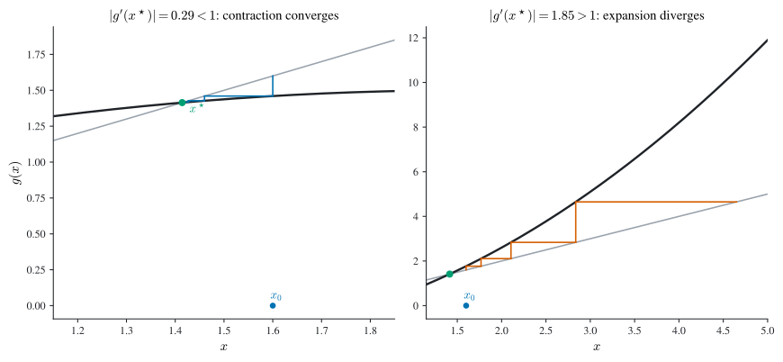
Before proving anything, it pays to watch both outcomes on the very map Equation 8.2. Take the scalar $F(x)=x^2-2$, whose positive root is $x^\star=\sqrt2\approx1.41421$, and iterate $g(x)=x-\eps F(x)$ from the same guess $x^{(0)}=1.6$ for two choices of $\eps$. The slope of $g$ at the root, $g'(x^\star)=1-\eps F'(x^\star)=1-2\sqrt2\,\eps$, decides everything: $\eps=0.25$ gives $g'(x^\star)\approx0.29$ (magnitude below $1$) and the iterates march into the root, while $\eps=-0.30$ gives $g'(x^\star)\approx1.85$ (magnitude above $1$) and they are thrown off to infinity, as Table 8.1 shows.

Table 8.1: Fixed-point iteration on $F(x)=x^2-2$ from $x^{(0)}=1.6$. Both columns share the fixed point $x^\star=\sqrt2$; only the step $\eps$, hence the slope $g'(x^\star)$, differs.

$k$	$x^{(k)}$, $\eps=0.25$ (converges)	$x^{(k)}$, $\eps=-0.30$ (diverges)
$0$	$1.6$	$1.6$
$1$	$1.46$	$1.768$
$2$	$1.4271$	$2.10575$
$3$	$1.41795$	$2.83601$
$4$	$1.41530$	$4.64886$

The same split is geometric in Figure 8.1: staircasing between the graph of $g$ and the line $y=x$ spirals into the fixed point exactly when $|g'(x^\star)|<1$ and walks away from it when $|g'(x^\star)|>1$. The magnitude of that slope is the whole game; the next two sections turn the observation into the Banach theorem and a checkable Jacobian test.

Figure 8.1: Fixed-point cobwebs for $g(x)=x-\eps(x^2-2)$ from $x^{(0)}=1.6$, both with fixed point $x^\star=\sqrt2$. Left: $\eps=0.25$ makes $|g'(x^\star)|=0.29<1$, and the staircase closes on the root. Right: $\eps=-0.30$ makes $|g'(x^\star)|=1.85>1$, and the staircase walks off to infinity.

When does the iteration converge? The Banach theorem

A clean sufficient condition for Equation 8.3 to converge is that $g$ pulls every pair of points closer together. Fix a norm $\norm{\cdot}$ on $\R^n$ and let $\norm{\cdot}$ also denote the induced operator norm on $\R^{n\times n}$.

Definition 8.2 (Contraction map) A map $g:\R^n\to\R^n$ is a contraction with parameter $k\in[0,1)$ if \[ \norm{g(x)-g(y)}\le k\,\norm{x-y}\qquad\text{for all }x,y\in\R^n . \tag{8.4}\]

This is a Lipschitz condition with constant below $1$: $g$ shrinks every distance by at least the fixed factor $k$. The proof leans on one analytic fact. Call $\{x^{(k)}\}$ Cauchy if for every $\eps>0$ there is $K$ with $\norm{x^{(k)}-x^{(l)}}\le\eps$ whenever $k,l\ge K$; the fact we use is that every Cauchy sequence in $\R^n$ converges: under any norm, $\R^n$ is complete.

Theorem 8.1 (Banach fixed-point theorem) Suppose $g:\R^n\to\R^n$ is a contraction with parameter $k\in[0,1)$. Let $x^{(0)}\in\R^n$ and set $x^{(k+1)}=g(x^{(k)})$ for $k=0,1,2,\dots$. Then:

the sequence converges, $x^{(k)}\to x^\star$ for some $x^\star\in\R^n$;
$x^\star$ is the unique fixed point of $g$ in $\R^n$; and
the error obeys \[ \norm{x^{(k)}-x^\star}\le\frac{k^{\,k}}{1-k}\,\norm{x^{(1)}-x^{(0)}}. \tag{8.5}\]

Read the bound Equation 8.5 carefully, since the letter $k$ plays two roles at once: it is the contraction constant and, in the exponent and the superscript $x^{(k)}$, the iteration count. After $k$ steps the error is at most $\tfrac{1}{1-k}$ times the contraction constant raised to the number of steps, times the length of the very first step.

Proof. Step 1: the iterates are Cauchy. For $k\le l$, telescoping and the triangle inequality give \[ \norm{x^{(k)}-x^{(l)}}=\Bigl\|\textstyle\sum_{i=k}^{l-1}\bigl(x^{(i)}-x^{(i+1)}\bigr)\Bigr\| \le\sum_{i=k}^{l-1}\norm{x^{(i)}-x^{(i+1)}}. \] Each summand shrinks geometrically. First, the $j$-fold composite $g^{j}$ is itself a contraction with parameter $k^{j}$: by induction, for $j\ge1$, \[ \norm{g^{j}(x)-g^{j}(y)}=\norm{g\bigl(g^{j-1}(x)\bigr)-g\bigl(g^{j-1}(y)\bigr)} \le k\,\norm{g^{j-1}(x)-g^{j-1}(y)}\le\cdots\le k^{j}\norm{x-y}. \] Since $x^{(i)}=g^{i}(x^{(0)})$ and $x^{(i+1)}=g^{i}(x^{(1)})$, \[ \norm{x^{(i)}-x^{(i+1)}}=\norm{g^{i}(x^{(0)})-g^{i}(x^{(1)})}\le k^{i}\norm{x^{(0)}-x^{(1)}}. \] Summing the geometric series and extending it to infinity, \[ \norm{x^{(k)}-x^{(l)}}\le\Bigl(\sum_{i=k}^{l-1}k^{i}\Bigr)\norm{x^{(0)}-x^{(1)}} \le\Bigl(\sum_{i=k}^{\infty}k^{i}\Bigr)\norm{x^{(0)}-x^{(1)}} =\frac{k^{\,k}}{1-k}\,\norm{x^{(0)}-x^{(1)}}. \tag{$\star$} \] The right side is free of $l$ and, because $k\in[0,1)$, tends to $0$ as $k\to\infty$; the sequence is Cauchy.

Step 2: convergence, uniqueness, and the bound. Being Cauchy in the complete space $\R^n$, the sequence has a limit $x^\star=\lim_k x^{(k)}$. A contraction is continuous, so Proposition 8.1 makes $x^\star$ a fixed point. It is the only one: two fixed points $x^\star,y^\star$ would satisfy $\norm{x^\star-y^\star}=\norm{g(x^\star)-g(y^\star)}\le k\norm{x^\star-y^\star}$, which forces $\norm{x^\star-y^\star}=0$ since $k<1$. Finally, hold $k$ fixed in $(\star)$ and send $l\to\infty$; continuity of the norm gives $\norm{x^{(k)}-x^{(l)}}\to\norm{x^{(k)}-x^\star}$, which is Equation 8.5. $\square$

Beyond mere convergence, Equation 8.5 is a genuine rate: the error decays geometrically, by the factor $k$ each step.

Linear convergence, in words

Since $\log\norm{x^{(k)}-x^\star}$ falls linearly in $k$ with slope $\log k<0$, this geometric decay is what numerical analysts call linear convergence, the $q=1$ case of Definition 8.5. Concretely, buying one more correct digit (a tenfold error cut) costs a roughly constant number of extra iterations, no matter how many digits you already have. Newton’s method will break that ceiling, gaining digits ever faster; that is the subject of Section 8.3.

A checkable test via the Jacobian

Verifying Equation 8.4 for every pair $x,y$ is awkward. A pointwise condition on first derivatives is far easier to check, and it goes through the Jacobian.

Definition 8.3 (Jacobian) For a vector field $g:\R^n\to\R^n$ with coordinate functions $g_1,\dots,g_n$, the Jacobian $Dg(x)$ is the $n\times n$ matrix-valued function \[ [Dg(x)]_{ij}=\pdiff{g_i}{x_j}(x). \]

Theorem 8.2 (Jacobian bound implies contraction) If there is $k\in[0,1)$ with $\norm{Dg(x)}\le k$ for all $x\in\R^n$ (induced norm matching the vector norm), then $g$ is a contraction with parameter $k$.

Proof. Fix $x,y$ and join them by the segment $z(t)=(1-t)x+ty$, $t\in[0,1]$, so $z(0)=x$, $z(1)=y$, and $z'(t)=y-x$. The fundamental theorem of calculus and the chain rule give \[ g(y)-g(x)=\int_0^1\diff{}{t}g(z(t))\,\dd t=\int_0^1 Dg(z(t))\,[y-x]\,\dd t. \] Taking norms and passing the triangle inequality through the integral, \[ \norm{g(y)-g(x)}\le\int_0^1\norm{Dg(z(t))\,[y-x]}\,\dd t \le\int_0^1\norm{Dg(z(t))}\,\norm{y-x}\,\dd t \le\int_0^1 k\,\norm{y-x}\,\dd t=k\,\norm{y-x}, \] using $\norm{Mv}\le\norm{M}\norm{v}$ and the hypothesis $\norm{Dg(z(t))}\le k$ along the segment. $\square$

The same “the update shrinks errors” as in Chapter 5

The condition $\norm{Dg(x)}\le k<1$ says the update map contracts errors by the factor $k$ every step. That is exactly the mechanism behind the stationary-iteration test $\spec(T)<1$ of Theorem 7.1: there the error propagates linearly through the iteration matrix $T$, and its spectral radius $\spec(T)$ (Definition 6.4) plays the role $k$ plays here. Linear solvers and nonlinear ones converge for the same reason (one application of the update shrinks the error), which is why both are governed by “how much below $1$” a single number sits.

Gradient descent as a contraction

Return to minimizing $u:\R^n\to\R$, i.e. solving $F(x)=\nabla u(x)=0$. Specializing the fixed-point map Equation 8.2 to $F=\nabla u$ and renaming the scalar $t>0$ (a step size) gives the update \[ x^{(k+1)}=x^{(k)}-t\,\nabla u(x^{(k)}), \tag{8.6}\] which is gradient descent. The contraction test tells us exactly when it converges and how fast.

Definition 8.4 (Strictly convex function) $u\in C^2(\R^n)$ is strictly convex if its Hessian $\nabla^2 u(x)=\bigl[\partial^2 u/\partial x_i\partial x_j\bigr]$ is positive definite for all $x$.

The $C^2$ assumption makes the Hessian exist and be symmetric (mixed partials commute); strict convexity is the same as every eigenvalue of $\nabla^2 u(x)$ being positive, and it forces any critical point to be the unique global minimizer. For a quantitative rate we ask for a uniform two-sided eigenvalue bound.

Standing assumption (strong convexity + Lipschitz gradient)

There are constants $0<c\le C$ with the eigenvalues of $\nabla^2 u(x)$ lying in $[c,C]$ for all $x$. The lower bound $c>0$ is strong convexity; the upper bound $C$ makes $\nabla u$ Lipschitz. The ratio $C/c$ is the condition number of the problem, it is exactly the $2$-norm condition number $\cond_2$ (Definition 4.6) of the positive-definite Hessian, largest eigenvalue over smallest, and it sets the speed below. This is the same conditioning that governed the linear solves of Chapters 4–5: a large $C/c$ means the level sets of $u$ are long, thin ellipsoids, the identical stretched geometry that made an ill-conditioned $Ax=b$ hard.

Theorem 8.3 (Gradient descent converges linearly) Under the standing assumption, gradient descent Equation 8.6 with step size $t=1/C$ converges to the unique global minimizer $x^\star$ of $u$. Moreover $g(x)=x-\tfrac1C\nabla u(x)$ is a contraction with parameter $k=1-c/C$, so by 1 \[ \ntwo{x^{(k)}-x^\star}\le\Bigl(1-\frac{c}{C}\Bigr)^{k}\frac{C}{c}\,\ntwo{x^{(1)}-x^{(0)}}. \tag{8.7}\]

Proof. By Theorem 8.2 it is enough to bound $\ntwo{Dg(x)}$. Differentiating $g(x)=x-\tfrac1C\nabla u(x)$, \[ Dg(x)=I_n-\frac1C\,\nabla^2 u(x). \] An eigenvalue $\lambda$ of $\nabla^2 u(x)$ becomes the eigenvalue $1-\lambda/C$ of $Dg(x)$. Since $c\le\lambda\le C$ gives $c/C\le\lambda/C\le1$, every eigenvalue of $Dg(x)$ lies in $[\,0,\,1-c/C\,]$. As $\nabla^2 u$ is symmetric, so is $Dg(x)$, and its $2$-norm equals its spectral radius (Definition 6.4), \[ \ntwo{Dg(x)}=\spec(Dg(x))=\max_i\abs{\lambda_i(Dg(x))}=1-\frac{c}{C}, \] the eigenvalues sitting in $[0,1-c/C]$ with $0\le1-c/C<1$. Thus $\ntwo{Dg(x)}\le k$ with $k=1-c/C\in[0,1)$, $g$ is a contraction, and 1 applies; Equation 8.7 is Equation 8.5 with $1/(1-k)=C/c$. $\square$

The step $t=1/C$ is safe, not optimal

Taking $t=1/C$ lands every eigenvalue of $Dg$ in $[0,1-c/C]$, which is convenient but not the fastest constant step. Balancing the two extreme eigenvalues instead, $t=2/(c+C)$, shrinks the contraction parameter to $(C-c)/(C+c)$, strictly below $1-c/C$ (for $C/c=10$ it is $0.818$ against $0.9$). Momentum and the conjugate-gradient acceleration of Chapter 5 (Theorem 8.3) push it further, toward $1-2\sqrt{c/C}$. So $1-c/C$ is a ceiling for the plainest gradient descent, not for first-order methods at large.

A concrete case makes the rate tangible. Minimize the quadratic \[ u(x)=\tfrac12 x^\top A x,\qquad A=\diag(1,10), \] whose gradient is $\nabla u(x)=Ax=(x_1,\,10x_2)$. The eigenvalues of the (constant) Hessian $A$ are $1$ and $10$, so $c=1$, $C=10$, the step is $t=1/C=0.1$, and the contraction parameter is $k=1-c/C=0.9$. The update reads \[ x^{(k+1)}=x^{(k)}-0.1\,(x_1^{(k)},\,10x_2^{(k)})=\bigl(0.9\,x_1^{(k)},\,0\bigr), \] because the stiff coordinate has $1-t\cdot10=0$: one step annihilates it. From $x^{(0)}=(1,1)$ the soft coordinate then decays by exactly $0.9$ each step while the stiff one stays pinned at $0$:

$k$	$x^{(k)}$	$\ntwo{x^{(k)}-x^\star}$
$0$	$(1,\,1)$	$\sqrt2\approx1.414$
$1$	$(0.9,\,0)$	$0.9$
$2$	$(0.81,\,0)$	$0.81$
$3$	$(0.729,\,0)$	$0.729$

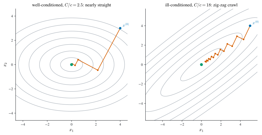
Here $x^\star=(0,0)$, and for $k\ge1$ we get $x^{(k)}=(0.9^{k},0)$ with $\ntwo{x^{(k)}-x^\star}=0.9^{k}$ exactly. The observed rate $0.9$ is precisely the predicted $k=1-c/C$, and Equation 8.7 holds with room to spare: its right-hand side is $0.9^{k}\cdot(C/c)\cdot\ntwo{x^{(1)}-x^{(0)}} =0.9^{k}\cdot10\cdot\sqrt{1.01}\approx10.05\cdot0.9^{k}$, comfortably above the true $0.9^{k}$. The lesson is written into the number $0.9$: a large condition number $C/c=10$ pushes the rate $1-c/C$ toward $1$, and the iteration crawls, the ill-conditioned line of Figure 8.3.

This clean diagonal run is in fact a best case, and it is worth seeing why before over-reading it. Because $A$ is aligned with the axes and $t=1/C$ zeroes the stiff coordinate outright, the residual “crawl” lives entirely in the soft coordinate, the one decaying at $0.9$; there is no zig-zag at all. The generic ill-conditioned picture is worse. When the Hessian’s eigenvectors are tilted off the coordinate axes, no single step size annihilates a coordinate, and the iterates zig-zag back and forth across the long axis of the ellipse while creeping toward the minimum (Figure 8.2). That is the same steepest-descent slowdown the conjugate-gradient method of Chapter 5 (Theorem 8.3) was built to cure. Plain gradient descent cannot escape it; escaping it is the motivation for the second-derivative method of the next section.

Figure 8.2: Steepest descent on the level sets of $u=\tfrac12 x^\top A x$. Left: a well-conditioned $A$ ($C/c=2.5$) has nearly round level sets, and the path drives almost straight to the minimum. Right: an ill-conditioned, tilted $A$ ($C/c=18$) has long thin ellipses, and the path zig-zags down the valley, crawling toward the center. Same rule, opposite geometry.

8.3 Superlinear iterations: Newton’s method

The second tier is where iterations accelerate. Instead of a constant per-step factor, the error is raised to a power $q>1$ each step, so the number of correct digits grows without bound per iteration. We first make “order of convergence” precise and prove the striking consequence (the error falls doubly exponentially) and then present Newton’s method as the worked instance that achieves $q=2$. Deferring the definition until now is deliberate: it is the organizing idea of the whole tier, not a footnote to any one algorithm.

How fast is fast: orders of convergence

Definition 8.5 (Order of convergence) Let an iterative method produce $x^{(k)}\to x^\star$. The method has order of convergence $q$ (a real number $q\ge1$) with rate $M>0$ if \[ \frac{\norm{x^{(k+1)}-x^\star}}{\norm{x^{(k)}-x^\star}^{q}}\le M \qquad\Longleftrightarrow\qquad \norm{x^{(k+1)}-x^\star}\le M\,\norm{x^{(k)}-x^\star}^{q} \tag{$*$} \] holds for all $k$. The case $q=1$ is linear convergence, $q>1$ is superlinear convergence, and $q=2$ is quadratic convergence.

The two regimes are not just quantitatively but qualitatively different, and the difference is all about the rate $M$.

Linear ($q=1$). Then $(*)$ reads $\norm{x^{(k+1)}-x^\star}\le M\norm{x^{(k)}-x^\star}$, and only $M<1$ forces the error down, otherwise the bound permits no progress, however close $x^{(0)}$ starts. So $M<1$ is a silent requirement when $q=1$, mirroring the role of $k$ in 1.
Superlinear ($q>1$). Now $M$ may exceed $1$ freely: provided $x^{(0)}$ lies close enough to $x^\star$, the inequality $(*)$ alone drags the error to zero. A superlinear method may dawdle far from the root and only reveal its speed once the iterate enters a neighborhood of $x^\star$; the definition captures this asymptotic behavior, not the transient.

Just how fast is superlinear? The next theorem answers precisely: the error decays like $e^{-\alpha q^{k}}$, doubly exponentially, since the exponent itself grows like $q^{k}$.

Theorem 8.4 (Superlinear convergence is doubly exponential) Suppose an iteration satisfies $(*)$ with $q>1$. If the initial error obeys $\norm{x^{(0)}-x^\star}<M^{-1/(q-1)}$, then the method converges, and there are constants $\alpha,C>0$ with \[ \norm{x^{(k)}-x^\star}\le C\,e^{-\alpha q^{k}} . \tag{8.8}\] One may take $C=M^{-1/(q-1)}$ and $\alpha=-\log\!\bigl(M^{1/(q-1)}\norm{x^{(0)}-x^\star}\bigr)$, which is positive precisely because the hypothesis is strict.

Proof. Write $E_k=\norm{x^{(k)}-x^\star}$, so $(*)$ is $E_{k+1}\le M E_k^{q}$. Logs turn the product into a linear recursion: $\log E_{k+1}\le b+q\log E_k$ with $b=\log M$. Define $a_0=\log E_0$, $a_{k+1}=b+q\,a_k$; then $\log E_k\le a_k$ for all $k$ by induction (the step is $\log E_{k+1}\le b+q\log E_k\le b+q a_k=a_{k+1}$). Solving the recursion, \[ a_k=q^{k}a_0+b\sum_{j=0}^{k-1}q^{j}=q^{k}a_0+b\,\frac{q^{k}-1}{q-1} =q^{k}\Bigl(a_0+\frac{b}{q-1}\Bigr)-\frac{b}{q-1}. \] Put $\alpha\defeq-\bigl(a_0+\tfrac{b}{q-1}\bigr)$. With $a_0=\log E_0$ and $b=\log M$, the condition $\alpha>0$ is $\log\!\bigl(E_0 M^{1/(q-1)}\bigr)<0$, i.e. $E_0<M^{-1/(q-1)}$, the hypothesis. Then $\log E_k\le a_k=-\alpha q^{k}-\tfrac{b}{q-1}$, and exponentiating gives $E_k\le C e^{-\alpha q^{k}}$ with $C=e^{-b/(q-1)}=M^{-1/(q-1)}$. Since $\alpha>0$ and $q>1$, the exponent $-\alpha q^{k}\to-\infty$ and $E_k\to0$. $\square$

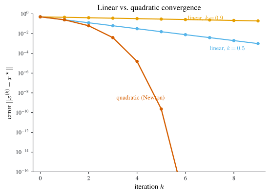
The contrast with the first tier is the whole point. Linear convergence adds a fixed number of correct digits per step; quadratic convergence roughly doubles the correct digits every step. Figure 8.3 draws both on a log scale, where linear convergence is a straight line, steeper when the contraction constant is smaller, and quadratic convergence peels away downward, each step bending it more sharply.

Figure 8.3: Error versus iteration count on a logarithmic scale. Linear convergence (1) plots as a straight line whose slope is set by the contraction constant $k$; a large condition number pushes $k$ toward $1$ and flattens the line. Quadratic convergence (Theorem 8.5) curves ever more steeply, each step roughly squares the error.

Newton’s method: linearize, then solve

Gradient descent used only first-order information and paid with a condition-number-limited linear rate. Newton’s method brings in the derivative of $F$ itself, and its logic is a two-move loop: replace $F$ near the current guess by its tangent (linear) approximation, then solve that linear problem exactly for the next guess.

Near $x^{(k)}$, the first-order multivariate Taylor expansion is \[ F(x)\approx F(x^{(k)})+DF(x^{(k)})\,(x-x^{(k)}), \] with $DF$ the Jacobian of $F$ (Definition 8.3, applied to $F$). Setting this linear model to zero, $0=F(x^{(k)})+DF(x^{(k)})(x-x^{(k)})$, and solving for $x$ (whenever $DF(x^{(k)})$ is invertible) names the next iterate, Newton’s method: \[ x^{(k+1)}=x^{(k)}-DF(x^{(k)})^{-1}F(x^{(k)}). \tag{8.9}\] For $n=1$ this is the schoolbook rule \[ x^{(k+1)}=x^{(k)}-\frac{F(x^{(k)})}{F'(x^{(k)})}. \] In optimization, $F=\nabla u$ has Jacobian $DF=\nabla^2 u$, so Newton minimizes $u$ by \[ x^{(k+1)}=x^{(k)}-\nabla^2 u(x^{(k)})^{-1}\nabla u(x^{(k)}), \] which for $n=1$ is $x^{(k+1)}=x^{(k)}-u'(x^{(k)})/u''(x^{(k)})$.

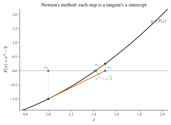
The two-move loop is pure tangent-following in one dimension: at $x^{(k)}$ the line $y=F(x^{(k)})+F'(x^{(k)})(x-x^{(k)})$ is the tangent to the graph of $F$, and its $x$-intercept is exactly the next iterate $x^{(k+1)}$. Figure 8.4 traces three such steps on $F(x)=x^2-2$: each tangent, dropped to the axis, hands its intercept to the next tangent, and the guesses close in fast on $x^\star=\sqrt2$. This is the geometric content the update equation Equation 8.9 hides.

Figure 8.4: Newton’s method on $F(x)=x^2-2$ from $x^{(0)}=1$. Each step replaces $F$ by its tangent at $(x^{(k)},F(x^{(k)}))$ (dotted drop line) and reads off $x^{(k+1)}$ as that tangent’s $x$-intercept. Three steps already reach $x^\star=\sqrt2$ to four digits.

One never actually forms $DF(x^{(k)})^{-1}$: inverting is $\bigO(n^3)$, potentially unstable, and wasteful. Instead the Newton step $y$ is found by solving a linear system, and that system is precisely the $Ax=b$ of Chapter 4: each Newton iteration is a linear solve, the exact callback promised in Section 8.1.

Algorithm: Newton’s method

Given $x^{(0)}$ and a maximum count $m$ (or a stopping tolerance):

set $x\leftarrow x^{(0)}$;
for $i=1,\dots,m$ (or until convergence):
1. assemble $A\leftarrow DF(x)$ and $b\leftarrow F(x)$;
2. solve the linear system $A\,y=b$ for the step $y$ (LU with partial pivoting, Chapter 4);
3. update $x\leftarrow x-y$;
4. optionally stop when $\norm{y}$ or $\norm{F(x)}$ falls below the tolerance.

So a Newton step costs one Jacobian evaluation and one linear solve. What repays that cost is the order of convergence, which we now show is $q=2$.

Newton’s quadratic rate

Theorem 8.5 (Local quadratic convergence of Newton’s method) Suppose the coordinate functions of $F:\R^n\to\R^n$ are all twice continuously differentiable. Let $x^\star$ solve $F(x)=0$ and suppose $DF(x^\star)$ is invertible. Then for any initial guess $x^{(0)}$ sufficiently close to $x^\star$, Newton’s method Equation 8.9 converges quadratically to $x^\star$.

Invertibility of $DF(x^\star)$ is a nondegeneracy hypothesis, and it is exactly what one expects to need. For $n=1$ it is $F'(x^\star)\neq0$, i.e. a simple root; for optimization ($F=\nabla u$) it demands $\nabla^2 u(x^\star)$ be invertible, i.e. $x^\star$ be a nondegenerate critical point (a strict local min, max, or saddle) rather than sit in a flat, degenerate valley. At a degenerate root the tangent model is too poor and the quadratic rate is lost.

Proof. We do the scalar case $n=1$; the vector case runs identically with multivariate Taylor expansion and matrix norms. Since $F'(x^\star)\neq0$ and $F'$ is continuous ($F\in C^2$), pick $\eps>0$ and $\delta>0$ with $\abs{F'(x)}\ge\eps$ on $I\defeq(x^\star-\delta,x^\star+\delta)$; and $F''$, continuous hence bounded, satisfies $\abs{F''(x)}\le C$ on $I$. Put $M\defeq C/(2\eps)$ and take $x^{(0)}$ close enough that $E_0=\abs{x^{(0)}-x^\star}<\min\{\delta,1/M\}$, so $x^{(0)}\in I$.

Assume inductively $x^{(k)}\in I$. Expand $F$ about $x^{(k)}$ to first order with Lagrange remainder and evaluate at $x^\star$: \[ F(x^\star)=F(x^{(k)})+F'(x^{(k)})\bigl(x^\star-x^{(k)}\bigr) +\tfrac12 F''(\xi^{(k)})\bigl(x^\star-x^{(k)}\bigr)^2, \] with $\xi^{(k)}$ between $x^\star$ and $x^{(k)}$, so $\xi^{(k)}\in I$. Using $F(x^\star)=0$ and $F'(x^{(k)})\neq0$, divide by $F'(x^{(k)})$ and rearrange: \[ -\frac{\tfrac12 F''(\xi^{(k)})(x^\star-x^{(k)})^2}{F'(x^{(k)})} =\frac{F(x^{(k)})}{F'(x^{(k)})}+\bigl(x^\star-x^{(k)}\bigr) =x^\star-\Bigl[x^{(k)}-\frac{F(x^{(k)})}{F'(x^{(k)})}\Bigr] =x^\star-x^{(k+1)}, \] the bracket being the Newton update Equation 8.9. Taking absolute values with $\abs{F''(\xi^{(k)})}\le C$ and $\abs{F'(x^{(k)})}\ge\eps$, \[ \abs{x^{(k+1)}-x^\star}\le\frac{C}{2\eps}\,\abs{x^{(k)}-x^\star}^2=M\,\abs{x^{(k)}-x^\star}^2, \] which is $(*)$ with $q=2$. Moreover $E_{k+1}\le M E_k^2=(M E_k)E_k\le(M E_0)E_k\le E_k$, so the error never grows and $x^{(k+1)}\in I$, closing the induction. With $(*)$ holding for all $k$ and $q=2>1$, Theorem 8.4 gives convergence, and the order is quadratic. $\square$

The rate is easiest to see on the simplest possible root. Take $F(x)=x^2-2$, whose positive root is $x^\star=\sqrt2=1.41421356\ldots$; Newton’s rule collapses to the ancient averaging iteration \[ x_{k+1}=x_k-\frac{x_k^2-2}{2x_k}=\frac12\Bigl(x_k+\frac{2}{x_k}\Bigr). \] Starting from $x_0=1$:

$k$	$x_k$	$\abs{x_k-\sqrt2}$
$0$	$1$	$4.14\times10^{-1}$
$1$	$1.5$	$8.58\times10^{-2}$
$2$	$1.41666667$	$2.45\times10^{-3}$
$3$	$1.41421569$	$2.12\times10^{-6}$
$4$	$1.41421356$	$1.59\times10^{-12}$

Read the error column: the exponents $-1,-2,-3,-6,-12$ roughly double once the iteration warms up, quadratic convergence doubling the correct digits each step, exactly as Theorem 8.4 promises for $q=2$. The rate constant is $M=\abs{F''(x^\star)}/\bigl(2\abs{F'(x^\star)}\bigr) =2/(2\cdot2\sqrt2)=1/(2\sqrt2)\approx0.354$, and the numbers obey $(*)$ tightly: for instance $M\cdot(2.45\times10^{-3})^2\approx2.1\times10^{-6}$, matching $\abs{x_3-\sqrt2}$, and indeed the ratio $\abs{x_{k+1}-\sqrt2}/\abs{x_k-\sqrt2}^2$ marches toward $0.354$ as $k$ grows.

Quadratic convergence is the payoff for Newton’s per-step cost: from a decent start, a handful of steps reach machine precision, where a linear method would still be grinding out digits one batch at a time. The prices are locality (a poor guess can diverge) and the need for a Jacobian and a linear solve each step. Both are addressed by globalization strategies and by quasi-Newton methods, which build up an approximate $DF$ from successive function values, and the wider optimization toolkit (Lagrangian duality, augmented-Lagrangian/ADMM splitting, and the rest) lies beyond our scope.

The chapter’s three workhorses now line up along the single tradeoff that organized it: more derivative information per step buys a higher order of convergence (Table 8.2).

Table 8.2: The three iterations sorted by order and per-step cost. The linear methods differ only in what plays the contraction constant ($\norm{Dg}$ directly, or $1-c/C$ through the conditioning); Newton pays a Jacobian and a solve each step and is repaid with $q=2$.

method	order $q$	derivative info per step	per-step cost	convergence condition
fixed-point iteration	$1$	$F$ only, via $g=x-\eps F$	one $g$ evaluation	$\norm{Dg(x)}\le k<1$ (Theorem 8.2)
gradient descent	$1$	gradient $\nabla u$	one gradient	strong convexity; rate set by $C/c$ (Theorem 8.3)
Newton’s method	$2$	Jacobian $DF$, then a linear solve	one Jacobian + one $n\times n$ solve	$x^{(0)}$ near $x^\star$, $DF(x^\star)$ invertible (Theorem 8.5)

8.4 Chapter summary

A nonlinear system $F(x)=0$ with $F:\R^n\to\R^n$ (Equation 8.1) has no direct solver, so we iterate. Linear systems ($F=Ax-b$) and optimization ($F=\nabla u$, best-behaved when $u$ is strictly convex, Definition 8.4) are the two anchoring special cases; the chapter sorts its iterations by order of convergence (Definition 8.5).
Tier A: linearly convergent ($q=1$). Fixed-point iteration $x^{(k+1)}=g(x^{(k)})$ recasts roots of $F$ as fixed points of $g(x)=x-\eps F(x)$ (Definition 8.1), and a convergent iteration must land on a fixed point (Proposition 8.1). The Banach fixed-point theorem
1. makes a contraction (Definition 8.2, parameter $k<1$) converge to its unique fixed point with error decaying like $k^{k}$ (Equation 8.5); the checkable test is $\norm{Dg(x)}\le k<1$ (Theorem 8.2), the same “update shrinks errors” as the $\spec(T)<1$ test of Theorem 7.1. Gradient descent with step $t=1/C$ is a contraction of parameter $1-c/C$ (Theorem 8.3); the condition number $C/c$ sets the rate, and a large one makes it slow, as the $A=\diag(1,10)$ example, with exact rate $0.9$, shows.
Tier B: superlinearly convergent ($q>1$). For $q>1$ the error falls doubly exponentially, $\bigO(e^{-\alpha q^{k}})$ (Theorem 8.4), so each step gains ever more digits. Newton’s method (Equation 8.9) is the archetype: it linearizes $F$ and solves the linear system $DF(x)\,y=F(x)$ each step, converging quadratically near a root where $DF(x^\star)$ is invertible (Theorem 8.5), doubling the correct digits per step, as the $\sqrt2$ example makes visible (Figure 8.3).

\(k\)	\(x^{(k)}\), \(\eps=0.25\) (converges)	\(x^{(k)}\), \(\eps=-0.30\) (diverges)
\(0\)	\(1.6\)	\(1.6\)
\(1\)	\(1.46\)	\(1.768\)
\(2\)	\(1.4271\)	\(2.10575\)
\(3\)	\(1.41795\)	\(2.83601\)
\(4\)	\(1.41530\)	\(4.64886\)

\(k\)	\(x^{(k)}\)	\(\ntwo{x^{(k)}-x^\star}\)
\(0\)	\((1,\,1)\)	\(\sqrt2\approx1.414\)
\(1\)	\((0.9,\,0)\)	\(0.9\)
\(2\)	\((0.81,\,0)\)	\(0.81\)
\(3\)	\((0.729,\,0)\)	\(0.729\)

\(k\)	\(x_k\)	\(\abs{x_k-\sqrt2}\)
\(0\)	\(1\)	\(4.14\times10^{-1}\)
\(1\)	\(1.5\)	\(8.58\times10^{-2}\)
\(2\)	\(1.41666667\)	\(2.45\times10^{-3}\)
\(3\)	\(1.41421569\)	\(2.12\times10^{-6}\)
\(4\)	\(1.41421356\)	\(1.59\times10^{-12}\)

method	order \(q\)	derivative info per step	per-step cost	convergence condition
fixed-point iteration	\(1\)	\(F\) only, via \(g=x-\eps F\)	one \(g\) evaluation	\(\norm{Dg(x)}\le k<1\) (Theorem 8.2)
gradient descent	\(1\)	gradient \(\nabla u\)	one gradient	strong convexity; rate set by \(C/c\) (Theorem 8.3)
Newton’s method	\(2\)	Jacobian \(DF\), then a linear solve	one Jacobian + one \(n\times n\) solve	\(x^{(0)}\) near \(x^\star\), \(DF(x^\star)\) invertible (Theorem 8.5)