7 Eigenvalue Problems
\[ \newcommand{\R}{\mathbb{R}} \newcommand{\C}{\mathbb{C}} \newcommand{\N}{\mathbb{N}} \newcommand{\E}{\mathbb{E}} \newcommand{\eps}{\varepsilon} \newcommand{\abs}[1]{\left\lvert #1 \right\rvert} \newcommand{\norm}[1]{\left\lVert #1 \right\rVert} \newcommand{\ninf}[1]{\left\lVert #1 \right\rVert_{\infty}} \newcommand{\ntwo}[1]{\left\lVert #1 \right\rVert_{2}} \newcommand{\none}[1]{\left\lVert #1 \right\rVert_{1}} \newcommand{\inner}[2]{\left\langle #1,\, #2 \right\rangle} \newcommand{\bigO}{\mathcal{O}} \newcommand{\dd}{\mathrm{d}} \newcommand{\diff}[2]{\frac{\mathrm{d} #1}{\mathrm{d} #2}} \newcommand{\pdiff}[2]{\frac{\partial #1}{\partial #2}} \newcommand{\spec}{\rho} \newcommand{\cond}{\kappa} \newcommand{\Span}{\operatorname{span}} \newcommand{\rank}{\operatorname{rank}} \newcommand{\tr}{\operatorname{tr}} \newcommand{\diag}{\operatorname{diag}} \newcommand{\argmax}{\operatorname*{arg\,max}} \newcommand{\argmin}{\operatorname*{arg\,min}} \newcommand{\defeq}{:=} \]
The characteristic polynomial \(\det(A-\lambda I)=0\) is how eigenvalues are defined; it is a poor way to compute them. Root-finding on a degree-\(n\) polynomial is badly conditioned in the coefficients, and simply assembling that polynomial already costs an \(\bigO(n^3)\) diagonalization, the very thing we hoped to dodge. The escape is to notice that we seldom want the entire spectrum. A few extreme eigenpairs are enough to answer the questions that actually come up: the equilibrium of a Markov chain, the ranking of a web graph, the leading directions of a data cloud, a low-rank compression of a matrix, a partition of a point set into clusters. This chapter is built around one primitive, the matrix–vector product, and shows how far it goes. A single engine, the power method, extracts the dominant eigenpair; blocking it gives subspace iteration, which extracts a dominant subspace; and that subspace machinery, in turn, drives the applications.
Throughout, \(A\in\R^{n\times n}\) has eigenvalues \(\lambda_1,\dots,\lambda_n\) and eigenvectors \(v_1,\dots,v_n\); \(\spec(A)=\max_i\abs{\lambda_i}\) is the spectral radius (Definition 6.4), and \(\sigma_1\ge\sigma_2\ge\dots\ge0\) are singular values. Norms, the condition number \(\cond(A)\) (Definition 4.6), and the matrix factorizations of Chapter 4 are used freely, with the symbol conventions of Notation: \(Q,R\) for orthonormal/triangular factors, and \(U\Sigma V^\top\) reserved for the SVD.
7.1 The power method
Everything in this chapter grows from one question: given only the ability to apply \(A\) to a vector, how do we find the direction \(A\) stretches the most? That direction is the eigenvector of largest eigenvalue, and the power method finds it by doing the obvious thing: apply \(A\), and apply it again. Notably it never inspects the entries of \(A\); it needs only a routine that returns \(Au\) from \(u\) (a matvec). When a matvec is cheap (\(A\) sparse, or sparse-plus-low-rank, costing \(\bigO(n)\) per apply), a handful of eigenpairs come out in \(\bigO(n)\) work, where a full diagonalization would spend \(\bigO(n^3)\).
The idea and why it converges
Take any \(x\in\R^n\) and watch \(Ax, A^2x, A^3x,\dots\). Left alone this sequence either explodes or decays to zero, so it has no useful limit; but its direction does settle, and rescaling to unit length each step exposes that direction. Suppose \(A\) is diagonalizable with a strictly dominant eigenpair \((\lambda_1,v_1)\): \[ \abs{\lambda_1}>\abs{\lambda_2}\ge\dots\ge\abs{\lambda_n}. \tag{7.1}\] When \(A\) is real this forces \(\lambda_1\) to be real, a complex \(\lambda_1\) would arrive with its conjugate \(\bar\lambda_1\) of equal modulus, contradicting strict dominance. Expand the seed in the eigenbasis, \(x=\sum_{i=1}^n c_iv_i\). Then \[ A^kx=\sum_{i=1}^n c_i\lambda_i^k v_i, \qquad \lambda_1^{-k}A^kx=c_1v_1+\sum_{i=2}^n c_i\Bigl(\tfrac{\lambda_i}{\lambda_1}\Bigr)^k v_i . \] Each ratio \(\abs{\lambda_i/\lambda_1}<1\) for \(i\ge2\), so every term but the first dies geometrically and \(\lambda_1^{-k}A^kx\to c_1v_1\). The one thing that can spoil this is \(c_1=0\), i.e. a seed exactly orthogonal (in the eigenbasis sense) to \(v_1\). That is a measure-zero accident: a seed drawn at random has \(c_1\ne0\) with probability one, so in practice we simply start random and never worry about it.
We do not know \(\lambda_1\), so we cannot literally divide by \(\lambda_1^k\). Instead we rescale to unit length, which removes whatever the dominant term’s magnitude happens to be: \[ u^{(k)}\defeq\frac{A^kx}{\ntwo{A^kx}} . \tag{7.2}\] Pulling the dominant term out of numerator and denominator, \[ u^{(k)}=\frac{\sum_i c_i\lambda_i^k v_i}{\bigl\lVert\sum_i c_i\lambda_i^k v_i\bigr\rVert} \;\longrightarrow\; \underbrace{\frac{c_1}{\abs{c_1}}\Bigl(\frac{\lambda_1}{\abs{\lambda_1}}\Bigr)^k}_{=:z^{(k)}} \,\frac{v_1}{\ntwo{v_1}}, \] with \(\abs{z^{(k)}}=1\) (so \(z^{(k)}=\pm1\) in the real case). The unit factor \(z^{(k)}\) is the unavoidable sign/phase wobble of an eigenvector, which is only ever defined up to scaling; the direction is what converges.
Theorem 7.1 (Power method convergence) Let \(A\in\R^{n\times n}\) be diagonalizable with a strictly dominant eigenpair \((\lambda_1,v_1)\) as in Equation 7.1, and let \(x=\sum_i c_iv_i\) with \(c_1\ne0\). With \(u^{(k)}\) as in Equation 7.2 there exist unit scalars \(z^{(k)}\) (\(z^{(k)}=\pm1\) when \(A\) is real) such that \[ \lim_{k\to\infty}\frac{u^{(k)}}{z^{(k)}}=\frac{v_1}{\ntwo{v_1}} . \] The convergence is geometric: the error decays like \(\bigl(\abs{\lambda_2}/\abs{\lambda_1}\bigr)^k\). The rate is the ratio \(\abs{\lambda_2/\lambda_1}\); the absolute spectral gap \(\abs{\lambda_1}-\abs{\lambda_2}\) sets that rate only after normalizing by \(\abs{\lambda_1}\), since \(\abs{\lambda_2/\lambda_1}=1-(\abs{\lambda_1}-\abs{\lambda_2})/\abs{\lambda_1}\).
Proof. The displayed limit is the computation above: \(\lambda_1^{-k}A^kx\to c_1v_1\) term by term, and dividing by \(\ntwo{A^kx}\) cancels the divergent scale \(\abs{\lambda_1}^k\abs{c_1}\) while leaving the unit factor \(z^{(k)}\). The rate is set by the slowest-vanishing surviving term, \(\abs{\lambda_2/\lambda_1}^k\), which dominates the deviation \(u^{(k)}-z^{(k)}v_1/\ntwo{v_1}\). \(\square\)
Figure 7.1 confirms the rate: a gap ratio \(\abs{\lambda_2/\lambda_1}=0.5\) buys about one digit every two steps, while \(0.9\) barely moves. The method survives loss of diagonalizability too, as long as a strictly dominant eigenvector exists, the argument then routes through the Jordan form and is fussier, but the conclusion is the same.
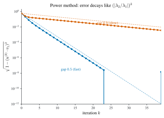
Why should renormalizing a divergent sequence produce a convergent one? Because the two behaviours live in different quantities. The magnitude \(\ntwo{A^kx}\sim\abs{\lambda_1}^k\) is what blows up or collapses; the direction is what we keep, and its distance to \(v_1\) shrinks by the factor \(\abs{\lambda_2/\lambda_1}\) each step. Dividing by the norm throws away the runaway magnitude and keeps the informative direction. The gap ratio is the speedometer: near \(1\) (eigenvalues bunched at the top) the needle barely moves; near \(0\) (one eigenvalue far out front) it races.
Estimating the eigenvalue and stopping
To stop we want a residual, ideally the relative norm \(\ntwo{Au^{(k)}-\lambda_1u^{(k)}}/\abs{\lambda_1}\), but that needs \(\lambda_1\), which we do not have. Given an eigenvector estimate \(u\), the matching eigenvalue falls out of the Rayleigh quotient: if \(Au=\lambda u\) then \(u^\top Au=\lambda\ntwo{u}^2\), so \[ \lambda=\frac{u^\top Au}{\ntwo{u}^2}, \qquad\text{and for unit }u,\quad \lambda=u^\top Au . \tag{7.3}\] This gives the running estimate \(\lambda_1^{(k)}=u^{(k)}\cdot(Au^{(k)})\) and a computable stopping test \(\ntwo{Au^{(k)}-\lambda_1^{(k)}u^{(k)}}/\abs{\lambda_1^{(k)}}\le\eps\).
Given a seed \(x^{(0)}\in\R^n\), a matvec routine for \(A\), a cap \(m\), and a tolerance \(\eps\). For \(k=0,1,\dots,m\):
- Normalize: \(u^{(k)}\leftarrow x^{(k)}/\ntwo{x^{(k)}}\).
- Matvec: \(x^{(k+1)}\leftarrow Au^{(k)}\).
- Rayleigh-quotient estimate: \(\lambda_1^{(k)}\leftarrow u^{(k)}\cdot x^{(k+1)}\).
- If \(\ntwo{x^{(k+1)}-\lambda_1^{(k)}u^{(k)}}/\abs{\lambda_1^{(k)}}\le\eps\), break.
Return \((\lambda_1^{(k)},u^{(k)})\). Each step is one matvec plus \(\bigO(n)\) work.
A worked run
Take the symmetric \[ A=\begin{pmatrix}2&1\\1&2\end{pmatrix}, \qquad \lambda_1=3,\ v_1=\tfrac1{\sqrt2}(1,1)^\top,\qquad \lambda_2=1,\ v_2=\tfrac1{\sqrt2}(1,-1)^\top, \] and seed \(x^{(0)}=(1,0)^\top\). The Rayleigh-quotient estimates \(\lambda_1^{(k)}=u^{(k)}\cdot Au^{(k)}\) run \[ 2.000,\quad 2.800,\quad 2.976,\quad 2.997,\quad \to 3 . \] Two rates coexist here. The eigenvector direction converges at the raw ratio \(\abs{\lambda_2/\lambda_1}=1/3\) (this is the quantity Figure 7.1 tracks for other spectra). The eigenvalue estimate converges faster, at the squared rate \((\lambda_2/\lambda_1)^2=1/9\) per step: the error sequence \(1,\,0.2,\,0.024,\,0.0027\) shrinks by roughly \(1/9\) each time. The squaring is no accident, for a symmetric matrix the Rayleigh quotient Equation 7.3 is stationary at an eigenvector, so a first-order error in the direction shows up only to second order in the estimate. That free extra digit is the reason we monitor \(\lambda_1^{(k)}\) rather than the direction.
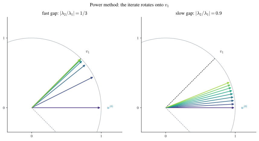
Figure 7.2 shows the underlying geometry: the normalized iterate is a point on the unit circle, and each matvec swings it toward \(v_1\). On this matrix (ratio \(1/3\)) the arrows bunch up on \(v_1\) within a handful of steps; on a nearly tied spectrum (ratio \(0.9\)) they crawl, exactly as the rate predicts.
The power method is a linearly convergent iteration in the sense of Definition 8.5: the error contracts by a constant factor \(\abs{\lambda_2/\lambda_1}<1\) every step (order \(q=1\)). That is the same regime as the stationary linear solvers of Chapter 5 and slower than the quadratic order \(q=2\) of Newton’s method in Section 8.3. The trade is deliberate: each step here is a single matvec, with no derivatives and no linear solves, so a slow-but-cheap iteration is exactly what a large sparse \(A\) wants.
The power method finds the extreme eigenvalue of whatever operator it is fed, so we can aim it elsewhere by feeding it a transformed matrix, all of which share the eigenvectors of \(A\). A shift \(A-\mu I\) moves the spectrum by \(\mu\) (eigenvalues \(\lambda_i-\mu\)); an inverse \((A-\mu I)^{-1}\) has eigenvalues \(1/(\lambda_i-\mu)\), so its dominant eigenpair is the one with \(\lambda_i\) nearest the shift \(\mu\). This is inverse iteration: pick \(\mu\) near the eigenvalue you want and run the power method on \((A-\mu I)^{-1}\), applying it by solving \((A-\mu I)y=u\) each step instead of a matvec. Taking \(\mu=0\) retargets to the eigenvalue of smallest modulus. The same idea recurs at the block level in Section 7.6.3, where running subspace iteration on \(2I-\hat L\) (a shift, then extreme end) picks out the smallest eigenpairs of the Laplacian \(\hat L\).
One dominant eigenvector is often not the whole story: PCA wants the top few directions, clustering the bottom few. The fix is to run the power method on a block of vectors at once, which is the subject of the next section.
7.2 Subspace iteration: the block power method
To capture a \(k\)-dimensional dominant subspace instead of a single direction, iterate the power method on \(k\) vectors simultaneously and keep them from collapsing onto the same dominant direction by reorthonormalizing after every apply. This is subspace iteration; together with the Rayleigh–Ritz step at the end, it is the workhorse behind PCA, the randomized SVD, and spectral clustering.
Basic algorithm
Let \(A\in\R^{n\times n}\) be diagonalizable, order its eigenvalues by modulus, and assume a spectral gap after the \(k\)-th: \[ \abs{\lambda_1}\ge\dots\ge\abs{\lambda_k}>\abs{\lambda_{k+1}}\ge\dots\ge\abs{\lambda_n}. \tag{7.4}\] Collect the leading eigenvectors into \(V_\star=[v_1,\dots,v_k]\in\R^{n\times k}\) (not orthonormal in general, since \(A\) need not be symmetric); we want the subspace \(\Span(V_\star)\). Start from a block \(Z=[z_1,\dots,z_k]\in\R^{n\times k}\).
Theorem 7.2 (Subspace iteration convergence) For a generic block \(Z\in\R^{n\times k}\) there is a sequence of invertible \(C_l\in\R^{k\times k}\) with \[ \lim_{l\to\infty}A^lZC_l=V_\star . \] Hence \(\Span(A^lZ)\to\Span(V_\star)\) as a subspace, even though \(A^lZ\) itself has no limit.
The precise genericity condition and the matrices \(C_l\) appear in the proof (Section 7.2.2). Forming \(A^lZ\) literally would overflow, so the practical iteration reorthonormalizes the block each step, the block version of the power method’s normalization. Write \(Q\) for an orthonormal basis of \(\Span(Z)\) (from Gram–Schmidt, a thin QR factorization \(Z=QR\), or Matlab’s orth):
Given a generic \(Z\in\R^{n\times k}\), matvec access to \(A\), and a cap \(m\). Let \(Q\) have orthonormal columns spanning \(\Span(Z)\). For \(j=0,1,\dots,m\):
- \(Z\leftarrow AQ\) (this is \(k\) matvecs, one per column).
- Reorthonormalize: let \(Q\) have orthonormal columns spanning \(\Span(Z)\).
Return \(Q\). For \(m\) large, \(\Span(Q)\approx\Span(V_\star)\).
Each pass costs \(k\) matvecs plus an \(\bigO(nk^2)\) orthonormalization. Sparse \(A\) (with \(\bigO(n)\) nonzeros) makes the matvecs \(\bigO(nk)\); even dense they are \(\bigO(n^2k)\), against \(\bigO(n^3)\) for a full diagonalization when \(k\ll n\).
Convergence proof
Proof. Diagonalize \(A=S\Lambda S^{-1}\) with \(S=[v_1,\dots,v_n]=[\,V_\star\mid V_\star'\,]\) (so \(V_\star'=[v_{k+1},\dots,v_n]\)) and \[ \Lambda=\begin{pmatrix}\Lambda_1&0\\0&\Lambda_2\end{pmatrix}, \qquad \Lambda_1=\diag(\lambda_1,\dots,\lambda_k),\quad\Lambda_2=\diag(\lambda_{k+1},\dots,\lambda_n); \] the gap Equation 7.4 makes \(\Lambda_1\) invertible. Change coordinates to the eigenbasis by setting \(Y=S^{-1}Z=\binom{Y_1}{Y_2}\) with \(Y_1\) of size \(k\times k\).
Hypothesis (G). \(Y_1\) is invertible. Equivalently, the seed block \(Z\) has a full-rank projection onto the dominant eigenspace \(\Span(V_\star)\). A random \(Z\) satisfies (G) with probability one, exactly as \(c_1\ne0\) did for the single-vector method.
Choose \(C_l=Y_1^{-1}\Lambda_1^{-l}\) (invertible under (G)). Then \[ A^lZC_l=S\Lambda^lYC_l =S\begin{pmatrix}\Lambda_1^lY_1\\\Lambda_2^lY_2\end{pmatrix}Y_1^{-1}\Lambda_1^{-l} =S\begin{pmatrix}I_k\\ M_l\end{pmatrix}, \qquad M_l=\Lambda_2^l\,(Y_2Y_1^{-1})\,\Lambda_1^{-l}. \] Everything now rides on one step: the tail block \(M_l\) vanishes geometrically. Its entries are \[ (M_l)_{ij}=\Bigl(\tfrac{\lambda_{k+i}}{\lambda_j}\Bigr)^l (Y_2Y_1^{-1})_{ij}, \qquad \Bigl\lvert\tfrac{\lambda_{k+i}}{\lambda_j}\Bigr\rvert\le\frac{\abs{\lambda_{k+1}}}{\abs{\lambda_k}}<1 \] for \(i\ge1,\ j\le k\), so \(M_l\to0\) at rate \((\abs{\lambda_{k+1}}/\abs{\lambda_k})^l\). Therefore \(A^lZC_l\to S\binom{I_k}{0}=[\,V_\star\mid V_\star'\,]\binom{I_k}{0}=V_\star\). \(\square\)
The rate mirrors the power method’s: it is the gap ratio \(\abs{\lambda_{k+1}}/\abs{\lambda_k}\) across the cut, not any interior gap. Eigenvalues bunched inside the block are recovered together and cost nothing; only the separation between kept and discarded eigenvalues sets the speed.
A computable convergence test
To stop, we need to measure how far successive subspaces sit apart, and a subspace has no coordinates, only its orthogonal projector does. So compare projectors. For orthonormal bases \(Q,Q'\in\R^{n\times k}\) (\(Q^\top Q=Q'^\top Q'=I_k\)) of two candidate subspaces, write the projectors \(\Pi=QQ^\top\) and \(\Pi'=Q'Q'^\top\) and measure them in the Frobenius inner product \(\inner{X}{Y}_{\mathrm F}=\tr(X^\top Y)\).
Theorem 7.3 (Projector distance between subspaces) If \(Q,Q'\in\R^{n\times k}\) have orthonormal columns with projectors \(\Pi=QQ^\top\), \(\Pi'=Q'Q'^\top\), then \[ \norm{\Pi-\Pi'}_{\mathrm F}^2=2\Bigl(k-\norm{Q^\top Q'}_{\mathrm F}^2\Bigr), \qquad \frac{\norm{\Pi-\Pi'}_{\mathrm F}}{\norm{\Pi}_{\mathrm F}} =\sqrt2\,\sqrt{1-k^{-1}\norm{Q^\top Q'}_{\mathrm F}^2}. \]
Proof. Expand the squared Frobenius norm as the inner product of \(\Pi-\Pi'\) with itself: \[ \norm{\Pi-\Pi'}_{\mathrm F}^2 =\inner{\Pi}{\Pi}_{\mathrm F}-2\inner{\Pi}{\Pi'}_{\mathrm F}+\inner{\Pi'}{\Pi'}_{\mathrm F}. \] Each projector is symmetric and idempotent, so \(\inner{\Pi}{\Pi}_{\mathrm F}=\tr(\Pi^\top\Pi)=\tr(\Pi)\), and cycling the trace \(\tr(QQ^\top)=\tr(Q^\top Q)=\tr(I_k)=k\); likewise \(\inner{\Pi'}{\Pi'}_{\mathrm F}=k\). For the cross term, \[ \inner{\Pi}{\Pi'}_{\mathrm F}=\tr(QQ^\top Q'Q'^\top)=\tr\!\bigl((Q^\top Q')(Q^\top Q')^\top\bigr) =\norm{Q^\top Q'}_{\mathrm F}^2, \] again by cycling the trace to expose the small \(k\times k\) matrix \(Q^\top Q'\). Substituting gives the first identity; the second divides through by \(\norm{\Pi}_{\mathrm F}=\sqrt{k}\). \(\square\)
The point is cost. The distance is read off the tiny \(k\times k\) matrix \(Q^\top Q'\) in \(\bigO(nk^2)\), never assembling the \(n\times n\) projectors (which would cost \(\bigO(n^2k)\)).
Stopping test and full algorithm
Comparing the current basis \(Q\) against the freshly reorthonormalized \(Q'\) by this relative distance supplies the stopping test the bare loop was missing.
Given a generic \(Z\in\R^{n\times k}\), matvec access to \(A\), a cap \(m\), and tolerance \(\eps\). Let \(Q\) have orthonormal columns spanning \(\Span(Z)\). For \(j=0,1,\dots,m\):
- \(Z\leftarrow AQ\).
- Let \(Q'\) have orthonormal columns spanning \(\Span(Z)\).
- \(\delta\leftarrow\sqrt2\,\sqrt{1-k^{-1}\norm{Q^\top Q'}_{\mathrm F}^2}\).
- \(Q\leftarrow Q'\).
- If \(\delta<\eps\), break.
Return \(Q\), whose span approximates \(\Span(V_\star)\).
Recovering eigenpairs via Rayleigh–Ritz
Subspace iteration hands back a subspace, not eigenpairs. To turn one into the other, specialize to symmetric \(A\). By the spectral theorem, a symmetric \(A=A^\top\) has an orthonormal eigenbasis and real eigenvalues, so the dominant block \(V_\star=[v_1,\dots,v_k]\) can be taken orthonormal, and suppose the iteration has converged, \(\Span(Q)=\Span(V_\star)\) with \(Q^\top Q=I_k\). Scaling freedom and possible repeated eigenvalues make recovering \(V_\star\) itself hopeless; we settle for the exact eigenvalues \(\lambda_1,\dots,\lambda_k\) and some orthonormal eigenvectors, as a matrix equation, an orthonormal \(\widehat Q\) with \(A\widehat Q=\widehat Q\Lambda_1\), \(\Lambda_1=\diag(\lambda_1,\dots,\lambda_k)\). The trick is to compress \(A\) to the subspace, where it is only \(k\times k\), and diagonalize it there.
Definition 7.1 (Rayleigh–Ritz procedure) Given an orthonormal basis \(Q\in\R^{n\times k}\) of an (approximately) invariant subspace of a symmetric \(A\):
- Form the \(k\times k\) symmetric matrix \(\bar A=Q^\top AQ\) (the Rayleigh quotient of the block).
- Diagonalize it fully, \(\bar A=W\bar\Lambda W^\top\), with \(W\) orthogonal (\(k\times k\)) and \(\bar\Lambda\) diagonal, entries ordered by decreasing modulus. This costs \(\bigO(k^3)\), independent of \(n\).
- Return the Ritz values \(\bar\Lambda\) and Ritz vectors \(\widehat Q=QW\).
Both outputs are exact, not approximate, when the subspace is exactly invariant.
Theorem 7.4 (Exactness of Rayleigh–Ritz) If \(\Span(Q)=\Span(V_\star)\) for the dominant orthonormal eigenblock \(V_\star\) of a symmetric \(A\), then the Rayleigh–Ritz procedure yields \(\bar\Lambda=\Lambda_1\) and \(\widehat Q=QW\) satisfies \(A\widehat Q=\widehat Q\Lambda_1\).
Proof. Both \(Q\) and \(V_\star\) are orthonormal bases of the same subspace, so they are related by an orthogonal change of basis \(O=V_\star^\top Q\): indeed \(V_\star O=V_\star V_\star^\top Q=\Pi_{V_\star}Q=Q\) because \(\Pi_{V_\star}=V_\star V_\star^\top\) fixes \(\Span(V_\star)\supseteq\Span(Q)\), and \(O^\top O=Q^\top V_\star V_\star^\top Q=Q^\top Q=I_k\). Then \[ \bar A=Q^\top AQ=(V_\star O)^\top A(V_\star O)=O^\top(V_\star^\top AV_\star)O=O^\top\Lambda_1 O , \] using \(AV_\star=V_\star\Lambda_1\) and \(V_\star^\top V_\star=I_k\). Since \(O\) is orthogonal, \(\bar A=O^\top\Lambda_1O\) already exhibits a diagonalization of \(\bar A\) with eigenvalues \(\lambda_1,\dots,\lambda_k\); ordering both the same way forces \(\bar\Lambda=\Lambda_1\), the first claim. For the second, insert \(I_k=OO^\top\) and \(\bar A=W\bar\Lambda W^\top=O^\top\Lambda_1O\) into \(A\widehat Q\): \[ A\widehat Q=AQW=A(V_\star O)W=V_\star\Lambda_1OW =V_\star O\,(O^\top\Lambda_1O)\,W=V_\star O\bar AW =V_\star O\,(W\bar\Lambda W^\top)\,W=V_\star OW\bar\Lambda=(QW)\Lambda_1=\widehat Q\Lambda_1 , \] using \(W^\top W=I_k\) and \(\bar\Lambda=\Lambda_1\) at the last steps. \(\square\)
With the engine complete (a single dominant vector from the power method, a dominant subspace with exact eigenpairs from subspace iteration plus Rayleigh–Ritz), the rest of the chapter is applications.
7.3 When the dominant eigenvector is the answer: Markov chains
The first family of applications needs nothing beyond the single-vector power method, because for a specific matrix the dominant eigenvector is the quantity of interest. The cleanest example is a Markov chain’s equilibrium.
Consider a system with \(n\) states \(1,\dots,n\) hopping at random between discrete times. For each state \(j\) we know a column of probabilities \(p_j=(p_{1j},\dots,p_{nj})^\top\), where \(p_{ij}\) is the chance of landing in state \(i\) next given that we are in state \(j\) now, the future depends only on the present (the Markov property). Probabilities demand \(p_{ij}\ge0\) and \(\sum_i p_{ij}=1\) for every \(j\), the latter being \(\mathbf 1^\top p_j=1\) with \(\mathbf 1\) the all-ones vector.
Definition 7.2 (Column-stochastic matrix) \(P=(p_{ij})\) is (column) stochastic if \(P\ge0\) entrywise and \(P^\top\mathbf 1=\mathbf 1\) (every column sums to \(1\)). It is positive, written \(P>0\), if \(p_{ij}>0\) for all \(i,j\).
A vector \(\pi\in\R^n\) is a probability distribution if \(\pi\ge0\) and \(\mathbf 1^\top\pi=1\). The role of \(P\) is to march distributions forward in time.
Proposition 7.1 (Distributions evolve by \(P\)) If \(\pi\) is the distribution of the state \(X_t\) at time \(t\), then \(P\pi\) is its distribution at time \(t+1\).
Proof. Condition on the current state and use the Markov property: \[ \Pr(X_{t+1}=i)=\sum_{j=1}^n\Pr(X_{t+1}=i\mid X_t=j)\,\Pr(X_t=j)=\sum_{j=1}^n p_{ij}\pi_j=[P\pi]_i . \] And \(P\) keeps distributions distributions: \(\mathbf 1^\top(P\pi)=(P^\top\mathbf 1)^\top\pi=\mathbf 1^\top\pi=1\), with \(P\pi\ge0\) since \(P,\pi\ge0\). \(\square\)
So time evolution is repeated application of \(P\), and the object of interest is the long-run limit \(\pi_\infty=\lim_{k\to\infty}P^k\pi\). If it exists it is again a probability vector, and passing to the limit in \(\pi_{k+1}=P\pi_k\) makes it a fixed point, \[ \pi_\infty=P\pi_\infty , \tag{7.5}\] the equilibrium (or invariant) distribution. Two facts tie this back to Section 7.1. First, Equation 7.5 says \(\pi_\infty\) is an eigenvector of \(P\) with eigenvalue \(1\). Second, \(P^k\pi\) is exactly the (already-normalized) power-method sequence for \(P\). So the equilibrium is the dominant eigenvector, provided the power method’s hypotheses hold, which positivity guarantees.
Theorem 7.5 (Perron–Frobenius) Let \(P\) be a positive stochastic matrix. Then \(P\) has a strictly dominant eigenvalue equal to \(1\), whose eigenvector can be scaled to a probability distribution. Hence the power method converges to the invariant distribution \(\pi_\infty\).
We take Theorem 7.5 as given: positivity forces a unique largest-modulus eigenvalue with a positive eigenvector, a matrix-analysis result whose refinements weaken positivity to irreducibility and aperiodicity.
PageRank
The web is a directed graph: pages \(1,\dots,n\) and edges \(E\), where \((i,j)\in E\) means page \(i\) links to page \(j\), encoded by an adjacency matrix \(A\) with \(A_{ij}=1\) on edges and \(0\) otherwise. We want to rank pages by importance. Counting inbound links is too crude, a link from a prominent page ought to count more than a link from a backwater, so PageRank uses eigenvector centrality: a page is important if important pages link to it. That self-reference is precisely what an eigenvector resolves.
From links to a chain. Turn the nonnegative \(A\) into a stochastic matrix the standard way: normalize each column to sum to one. Assuming every page has an outgoing link (delete any that do not), define \(\tilde P\) by \[ \tilde P^\top=\diag(A\mathbf 1)^{-1}A, \qquad \tilde P_{ji}=\begin{cases}\dfrac{1}{\deg^-(i)}, & (i,j)\in E,\\[2pt] 0,&(i,j)\notin E,\end{cases} \tag{7.6}\] with \(\deg^-(i)\) the outdegree of page \(i\). The reading is a random walk: from the current page, follow a uniformly random outgoing link.
Damping. Plain \(\tilde P\) can converge slowly and dangling structure can break the hypotheses. The remedy is a damping factor \(\tau\in(0,1)\): with probability \(\tau\) follow a link, and with probability \(1-\tau\) teleport to a page chosen uniformly at random. This is the chain \[ P=\tau\tilde P+(1-\tau)\tfrac1n\mathbf 1\mathbf 1^\top , \tag{7.7}\] with \(\mathbf 1\mathbf 1^\top\) the all-ones matrix. Now \(P\) is stochastic and strictly positive, so Theorem 7.5 delivers a dominant eigenvector \(\pi^{\star}\) with eigenvalue \(1\); scaled to \(\pi^{\star}\ge0\), \(\mathbf 1^\top\pi^{\star}=1\), the entry \(\pi^{\star}_i\) is the PageRank of page \(i\), the long-run fraction of time the surfer spends there.
The PageRank of a page is not a score attached to the page in isolation; it is the fraction of eternity a random surfer spends parked there. High rank means “many walks lead here and linger,” which is why importance propagates: landing on a hub that points to you funnels dwell time your way. Teleportation (\(1-\tau\)) keeps the surfer from getting trapped in a corner of the web with no way out, guaranteeing every page gets some dwell time and making the equilibrium unique.
PageRank is the power method on \(P\) of Equation 7.7, only simpler: the dominant eigenvalue is exactly \(1\), so no renormalization is ever needed. Start from any distribution \(\pi^{(0)}\) and iterate \(\pi^{(k+1)}=P\pi^{(k)}\); each iterate stays a distribution and \(\pi^{(k)}\to\pi^{\star}\). The matrix \(P\) is never formed densely: the damping term acts as \(\tfrac{1-\tau}{n}(\mathbf 1^\top\pi^{(k)})\mathbf 1=\tfrac{1-\tau}{n}\mathbf 1\), so each step costs \(\bigO(\lvert E\rvert)\).
A three-page example. Let page \(1\) link to \(\{2,3\}\), page \(2\) to \(\{3\}\), and page \(3\) to \(\{1\}\), outdegrees \((2,1,1)\). Column-normalizing gives \[ \tilde P=\begin{pmatrix}0&0&1\\[2pt]\tfrac12&0&0\\[2pt]\tfrac12&1&0\end{pmatrix}, \] whose invariant distribution solves \(\tilde P\pi=\pi\): from the rows, \(\pi_1=\pi_3\) and \(\pi_2=\tfrac12\pi_1\), and normalizing \(\pi_1+\pi_2+\pi_3=1\) gives \[ \pi=(0.4,\ 0.2,\ 0.4). \] Damping with \(\tau=0.85\) (the classic choice) shifts this only slightly, to \[ \pi^\star=(0.388,\ 0.215,\ 0.397), \] mixing in the uniform teleport distribution \((\tfrac13,\tfrac13,\tfrac13)\), a small, stabilizing perturbation. Pages \(1\) and \(3\) tie in the undamped chain; damping breaks the tie faintly in favour of \(3\). Notice that page \(1\) keeps pace with page \(3\) despite having only one inbound link to page \(3\)’s two: its single backlink comes from page \(3\) itself, a high-rank page, so its importance is inherited, not counted. This is exactly the payoff of eigenvector centrality over raw link counting. Both vectors already sum to \(1\), illustrating why the PageRank iteration skips renormalization entirely.
7.4 Principal component analysis
The next two applications are about the SVD, so we recover directions from the top singular vectors rather than from eigenvectors of the matrix itself. Both lean on one optimality fact, worth stating once.
The decompositions PCA rests on
Every \(A\in\R^{m\times n}\) factors as \(A=U\Sigma V^\top\) with orthogonal \(U,V\) and \(\Sigma=\diag(\sigma_1,\sigma_2,\dots)\), \(\sigma_1\ge\sigma_2\ge\dots\ge0\), the SVD. The compact form keeps the \(r=\rank(A)\) positive singular values, \(A=\sum_{i=1}^r\sigma_iu_iv_i^\top\), and the truncated rank-\(k\) form keeps the top \(k\). The SVD is the spectral theorem wearing a disguise: \(A^\top A=V\Sigma^2V^\top\) and \(AA^\top=U\Sigma^2U^\top\), so the right and left singular vectors are eigenvectors of \(A^\top A\) and \(AA^\top\) with eigenvalues \(\sigma_i^2\), the observation that lets the eigen-engine compute an SVD. The one theorem we invoke is Eckart–Young–Mirsky: among all rank-\(k\) matrices, the truncated SVD is the closest to \(A\) in Frobenius norm. Everything below is that theorem applied.
The optimization and its solution
Given data points \(x_j\in\R^m\), \(j=1,\dots,n\), PCA seeks the \(k\)-dimensional subspace that best captures the cloud, in statistical terms, the one explaining the most variance. Assume the data is de-meaned, \(\frac1n\sum_j x_j=0\) (subtract the mean if not), and stack it into \(X=[x_1,\dots,x_n]\in\R^{m\times n}\), with empirical covariance \(\frac1n XX^\top\).
Describe a subspace by an orthonormal basis \(Q=[q_1,\dots,q_k]\), \(Q^\top Q=I_k\), with projector \(\Pi=QQ^\top\). Minimize the total squared distance of the data from the subspace, \[ f(Q)\defeq\sum_{j=1}^n\ntwo{x_j-\Pi x_j}^2 . \tag{7.8}\] Since \((I-QQ^\top)x_j\) is the \(j\)-th column of \((I-QQ^\top)X\) and the squared Frobenius norm sums squared column norms, \[ f(Q)=\bigl\lVert X-QQ^\top X\bigr\rVert_{\mathrm F}^2 . \] Now let \(X=\sum_{i=1}^r\sigma_iu_iv_i^\top\) be the compact SVD and \(\tilde X=\sum_{i=1}^k\sigma_iu_iv_i^\top\) its rank-\(k\) truncation, with \(\tilde U=[u_1,\dots,u_k]\). Because \(\rank(QQ^\top X)\le k\), Eckart–Young says no \(Q\) can bring \(QQ^\top X\) nearer to \(X\) than \(\tilde X\); and \(Q=\tilde U\) attains the bound, since \[ QQ^\top X=\tilde U\tilde U^\top\sum_{i=1}^r\sigma_iu_iv_i^\top=\sum_{i=1}^k\sigma_iu_iv_i^\top=\tilde X , \] using \(\tilde U^\top u_i=e_i\) for \(i\le k\) and \(0\) for \(i>k\). So the optimal subspace is the span of the top \(k\) left singular vectors of the de-meaned \(X\), equivalently, the span of the dominant \(k\) eigenvectors of the covariance \(\frac1n XX^\top\), which is exactly what subspace iteration on \(XX^\top\) returns.
For a point \(x_j\), the coordinate \(u_i\cdot x_j\) is its \(i\)-th principal component; the \(j\)-th column of \(Y=Q^\top X\in\R^{k\times n}\) collects the first \(k\). Reading \(Y\) as a compression \(\R^m\to\R^k\), we recover the data by \(\tilde X=QY=QQ^\top X\), and because \(Q\) minimized Equation 7.8 this recovery is as faithful as any \(k\)-dimensional linear compression can be.
A two-dimensional example
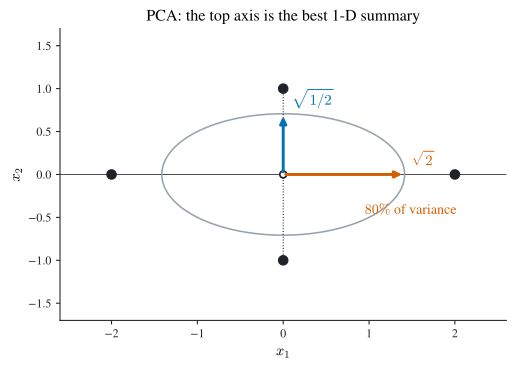
Take the four points \((2,0),(0,1),(-2,0),(0,-1)\). Their mean is \(0\), so no de-meaning is needed, and the data matrix and covariance are \[ X=\begin{pmatrix}2&0&-2&0\\0&1&0&-1\end{pmatrix}, \qquad \frac14 XX^\top=\frac14\begin{pmatrix}8&0\\0&2\end{pmatrix}=\begin{pmatrix}2&0\\0&\tfrac12\end{pmatrix}. \] The covariance is already diagonal, so the principal components are the coordinate axes: the first is the \(x\)-axis with variance \(2\), the second the \(y\)-axis with variance \(\tfrac12\). The top component captures \(2/(2+\tfrac12)=80\%\) of the total variance, so projecting these four points onto the \(x\)-axis, the span of the top left singular vector, is the best one-dimensional summary, keeping four fifths of the spread. Figure 7.3 draws the picture: the covariance ellipse has semi-axes \(\sqrt2\) and \(\sqrt{1/2}\) (the two standard deviations), the top axis is the long one, and dropping each point onto it loses only the short \(20\%\), which is precisely the residual Eckart–Young leaves behind.
7.5 Randomized SVD
Subspace iteration plus Rayleigh–Ritz already computes a truncated SVD: the top \(k\) left singular vectors of \(A\in\R^{m\times n}\) (\(m\ge n\)) are the dominant \(k\) eigenvectors of \(AA^\top\) (eigenvalues \(\sigma_i^2\)), the right ones the dominant \(k\) eigenvectors of \(A^\top A\). Here the eigen-engine’s letters line up on their own: the eigenvectors of \(AA^\top\) are the left singular vectors \(u_i\). But when the gap \(\sigma_k-\sigma_{k+1}\) is small the iteration crawls. The randomized SVD skips iteration altogether, trading it for a controlled error that shrinks with how fast the singular values decay.
The exact-rank warm-up
Suppose \(\rank(A)=k\) exactly. Draw a random \(Z=[z_1,\dots,z_k]\in\R^{n\times k}\). The images \(Az_1,\dots,Az_k\) lie in \(\operatorname{range}(A)\) and, with probability one, are independent, so they span it: \[ \Span(AZ)=\operatorname{range}(A)=\Span(u_1,\dots,u_k), \] the last equality because \(A=\sum_{i=1}^k\sigma_iu_iv_i^\top\) stops at \(k\). So a single random matvec block exposes the range, no iteration at all. Let \(X=\operatorname{orth}(AZ)\) span \(\Span(u_1,\dots, u_k)\). Feeding \(X\) to Rayleigh–Ritz on \(AA^\top\) recovers \(U\) and \(\Sigma\): form \(B=X^\top AA^\top X=(X^\top A)(X^\top A)^\top\), diagonalize \(B=W\bar\Lambda W^\top\), and set \(U=XW\), \(\Sigma=\sqrt{\bar\Lambda}\).
A slicker route delivers \(U\), \(\Sigma\), and \(V\) together. Draw a second random \(W_0\in\R^{m\times k}\) and let \(Y=\operatorname{orth}(A^\top W_0)\) span the row space. Since \(XX^\top A=A\) (as \(XX^\top\) projects onto \(\operatorname{range}(A)\)) and \(AYY^\top=A\), \[ A=XX^\top A=XX^\top AYY^\top=X(X^\top AY)Y^\top . \] Form the small \(\bar A=X^\top AY\in\R^{k\times k}\) (generally not symmetric), take its full SVD \(\bar A=\tilde U\tilde\Sigma\tilde V^\top\), and read off \(U=X\tilde U\), \(V=Y\tilde V\), \(\Sigma=\tilde\Sigma\). This agrees with the two-sided recipe, since \(\bar A\bar A^\top=X^\top AA^\top X=B\): the singular vectors of the tiny \(\bar A\) are the very eigenvectors Rayleigh–Ritz would produce.
Beyond rank \(k\)
Real matrices are rarely exactly rank \(k\). So oversample: draw \(\tilde k\ge k\) random vectors \(Z\in\R^{n\times\tilde k}\), \(W_0\in\R^{m\times\tilde k}\), so that \(\Span(AZ)\) and \(\Span(A^\top W_0)\) only approximately contain the ranges. With \(X=\operatorname{orth}(AZ)\), \(Y=\operatorname{orth}(A^\top W_0)\), \[ A\approx XX^\top A\approx XX^\top AYY^\top=X\bar AY^\top, \qquad \bar A=X^\top AY\in\R^{\tilde k\times\tilde k}. \] The error is controlled by the following, stated without proof (it is beyond this course; the one-line intuition is that oversampling makes \(\Span(AZ)\) capture the dominant singular directions with high probability, leaving only the tail energy \(\sum_{i>k}\sigma_i^2\)).
Theorem 7.6 (Randomized range approximation) Let \(\delta>0\), \(A\in\R^{m\times n}\), and \(X=\operatorname{orth}(AZ)\) with \(Z\in\R^{n\times\tilde k}\) having i.i.d. standard-normal entries. There is a universal constant \(C\) such that if \(\tilde k\ge C\,(k+\log(1/\delta))\), then with probability at least \(1-\delta\), \[ \bigl\lVert (I-XX^\top)A\bigr\rVert_{\mathrm F}^2\le 2\sum_{i>k}\sigma_i^2 , \] \(\sigma_i\) the singular values of \(A\). (Some sources print this as \(\lVert XX^\top A\rVert_{\mathrm F}\), the projection onto the range rather than the residual, which is \(\approx\lVert A\rVert_{\mathrm F}\), not small; the residual bound above is the one that matters.)
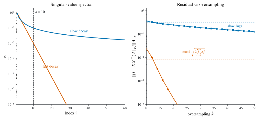
So when \(A\) has numerical rank \(k\), meaning \(\sum_{i>k}\sigma_i^2\) is negligible, oversampling to a small multiple of \(k\) makes the randomized SVD accurate with high probability. Figure 7.4 makes the rule of thumb operational: for a matrix with fast (geometric) singular decay the measured residual \(\norm{(I-XX^\top)A}_{\mathrm F}\) dives to the tail level \(\sqrt{2\sum_{i>k}\sigma_i^2}\) with only a handful of extra columns, while for slow (algebraic) decay the fat tail keeps the residual high and oversampling barely helps. Oversample a little; oversample more when the tail is fat.
Given matvec access to \(A\) and \(A^\top\), target rank \(k\), oversampling \(\tilde k\ge k\):
- Draw \(Z\in\R^{n\times\tilde k}\), \(W_0\in\R^{m\times\tilde k}\) with i.i.d. standard-normal entries.
- Form \(AZ\) and \(A^\top W_0\); orthonormalize the columns to get \(X\) and \(Y\).
- Form \(\bar A=X^\top AY\in\R^{\tilde k\times\tilde k}\) and take its full SVD \(\bar A=\tilde U\tilde\Sigma\tilde V^\top\).
- Recover \(\hat U=[X\tilde U]_{:,1:k}\), \(\hat V=[Y\tilde V]_{:,1:k}\), \(\hat\Sigma=[\tilde\Sigma]_{1:k,1:k}\).
Then \(A\approx\hat U\hat\Sigma\hat V^\top\) is an approximate rank-\(k\) truncated SVD.
7.6 Spectral clustering
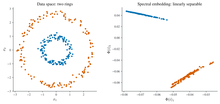
The last application partitions data into clusters that need not be linearly separable (two concentric rings, say) where \(k\)-means on the raw coordinates fails outright. The move is to re-embed the data using eigenvectors of a graph Laplacian, after which the clusters do separate (Figure 7.5). This time the informative eigenvectors are the ones with the smallest eigenvalues, so subspace iteration runs on a shifted matrix.
A weighted graph from data
Given \(x_1,\dots,x_n\in\R^m\), build a weighted graph whose edge weights measure similarity. A similarity kernel is a symmetric \(K(x,y)=K(y,x)\ge0\); the usual pick is the Gaussian kernel of width \(\sigma>0\), \[ K(x,y)=e^{-\frac{1}{2\sigma^2}\ntwo{x-y}^2}. \tag{7.9}\] This yields a symmetric weighted adjacency matrix \(A_{ij}=K(x_i,x_j)\), large for nearby points.
Graph Laplacians
Definition 7.3 (Graph Laplacian) For a weighted adjacency \(A\) with degree matrix \(D=\diag(A\mathbf 1)\) (so \(D_{ii}=\sum_j A_{ij}\)), the graph Laplacian is \(L=D-A\), i.e. \(L_{ij}=\delta_{ij}D_{ii}-A_{ij}\). Its symmetric normalized form is \[ \hat L=D^{-1/2}LD^{-1/2}=I-D^{-1/2}AD^{-1/2}, \qquad \hat L_{ij}=\delta_{ij}-\frac{A_{ij}}{\sqrt{D_{ii}D_{jj}}}. \tag{7.10}\]
Why the Laplacian encodes clusters is clearest through the left-normalized variant \(\tilde L=D^{-1}L=I-D^{-1}A\): for any \(v\), \[ [\tilde Lv]_i=v_i-\frac{\sum_j A_{ij}v_j}{\sum_j A_{ij}}, \] the gap between \(v_i\) and the weighted average of its neighbours, a discrete smoothness operator, small on functions that barely change across the graph. Three facts pin the spectrum: (1) \(L\mathbf 1=0\), so the constant vector is a null eigenvector; (2) \(L\) is diagonally dominant with nonnegative diagonal; hence (3) \(L\) is positive semidefinite. For \(\hat L\) one more bound holds.
Proposition 7.2 (Spectrum of the normalized Laplacian) The eigenvalues of \(\hat L=D^{-1/2}LD^{-1/2}\) all lie in \([0,2]\).
Proof. \(\hat L\) is positive semidefinite (congruent to the PSD \(L\) via \(D^{-1/2}(\cdot)D^{-1/2}\)), so its eigenvalues are \(\ge0\). For the upper bound, \(\hat L\) is similar to \(\tilde L=D^{-1}L\) (indeed \(\tilde L=D^{-1/2}\hat LD^{1/2}\)), so they share a spectrum, and \(\spec(\tilde L)\le\ninf{\tilde L}\). Each row of \(\tilde L\) has \(1\)-norm \[ \sum_{j}\Bigl\lvert\delta_{ij}-\tfrac{A_{ij}}{D_{ii}}\Bigr\rvert \le 1+\frac{1}{D_{ii}}\sum_j A_{ij}=1+\frac{D_{ii}}{D_{ii}}=2 , \] so \(\ninf{\tilde L}\le2\) and every eigenvalue of \(\hat L\) lies in \([0,2]\). \(\square\)
For PCA we wanted the top eigenvectors, the directions of most variance. For clustering we want the bottom eigenvectors of \(\hat L\), and the smoothness reading explains the reversal. A low-\(\hat L\) eigenvector is a graph function that changes little across strong edges, so it is nearly constant within a tightly-connected cluster and jumps only between clusters. Those functions are indicator-like: they label which cluster a vertex belongs to. The very lowest is the constant vector \(\mathbf 1\) (eigenvalue \(0\)), carrying no information; the next few carry the cluster structure.
Spectral embedding
A spectral embedding is a map \(\Phi:\{1,\dots,n\}\to\R^d\) sending vertex \(i\) (data point \(x_i\)) to a new point \(\Phi(i)\). Let \(Q=[v_1,\dots,v_d]\in\R^{n\times d}\) hold the orthonormal eigenvectors of the \(d\) lowest eigenvalues of \(\hat L\). Since we want the lowest eigenpairs, run subspace iteration on \(2I-\hat L\): its dominant eigenvectors are those of \(\hat L\)’s smallest eigenvalues, and this is valid precisely because \(\spec(\hat L)\subseteq[0,2]\) by Proposition 7.2 keeps \(2I-\hat L\) positive semidefinite. The embedding is \[ \Phi(i)=[Q_{i,:}]^\top\in\R^d , \] the \(i\)-th row of \(Q\). Points in one cluster land near one another in \(\R^d\) even when the original clusters interleave geometrically, which is what pulls apart the rings of Figure 7.5.
Clustering
Whether we cluster the raw \(x_i\in\R^m\) or the embedded \(y_i=\Phi(i)\in\R^d\) (the results differ, and the embedded version is the whole point), we split into \(k\) clusters with \(k\)-means. It posits centroids \(z_1,\dots,z_k\in\R^m\) and an assignment \(c:\{1,\dots,n\}\to\{1,\dots,k\}\), minimizing \[ F(z_1,\dots,z_k,c)=\sum_{j=1}^k\sum_{i:\,c(i)=j}\ntwo{x_i-z_j}^2 \tag{7.11}\] over both centroids and assignment.
From a random start, alternate the two closed-form minimizations until the assignment stops changing:
- Centroids (assignment fixed): \(z_j\leftarrow\dfrac{\sum_{i:\,c(i)=j}x_i}{\#\{i:c(i)=j\}}\), the cluster mean.
- Assignment (centroids fixed): \(c(i)\leftarrow\argmin_{j}\ntwo{x_i-z_j}^2\), the nearest centroid.
Each step can only lower Equation 7.11, so Lloyd’s algorithm never increases the objective and terminates, but with no guarantee of the global optimum: it can stall in a bad local minimum, and random restarts are the standard cure. Run on interleaved data it fails; run on the spectral embedding it succeeds, because the embedding has already converted “same cluster” into “nearby in \(\R^d\).”
7.7 One engine, four applications
Every application in this chapter is the same matvec engine pointed at a different matrix and a different end of its spectrum, as Table 7.1 collects. The only real choices are which matrix to apply, which eigenpairs you want, and whether they sit at the dominant or the smallest end (retargeted by a shift, as above).
| Problem | Matrix acted on | Eigenpairs wanted | End of spectrum | Engine |
|---|---|---|---|---|
| Markov / PageRank | chain \(P\) | eigenvalue \(1\) | dominant | power method |
| PCA | covariance \(XX^\top\) | top \(k\) | dominant | subspace iteration + Rayleigh–Ritz |
| Randomized SVD | \(AA^\top\) (and \(A^\top A\)) | top \(k\) | dominant | single random block (no iteration) |
| Spectral clustering | Laplacian \(\hat L\) | bottom \(k\) | smallest, via \(2I-\hat L\) | subspace iteration |
7.8 Chapter summary
- The power method (Theorem 7.1) finds the dominant eigenpair by normalized repeated matvecs \(u^{(k)}=A^kx/\ntwo{A^kx}\); it converges geometrically at rate \(\abs{\lambda_2/\lambda_1}\) set by the spectral gap, a linearly convergent iteration (Definition 8.5), with the eigenvalue read off the Rayleigh quotient Equation 7.3.
- Subspace iteration (Theorem 7.2) is the block power method with reorthonormalization; convergence is detected by the projector distance Theorem 7.3, and Rayleigh–Ritz
- recovers exact eigenpairs from the converged subspace when \(A\) is symmetric.
- A Markov chain advances distributions by a stochastic matrix \(P\) (Proposition 7.1); its invariant distribution is the eigenvalue-\(1\) dominant eigenvector, guaranteed and computable by the power method when \(P\) is positive (Perron–Frobenius, Theorem 7.5). PageRank is that method on the damped chain Equation 7.7, where the dominant eigenvalue is exactly \(1\) so no renormalization is needed.
- PCA minimizes Equation 7.8; the optimal \(k\)-dimensional subspace is the span of the top \(k\) left singular vectors of the de-meaned data (Eckart–Young), the dominant eigenvectors of the covariance.
- The randomized SVD approximates the rank-\(k\) truncated SVD from a few random matvecs, exact when \(\rank(A)=k\) and accurate up to the tail \(\sum_{i>k}\sigma_i^2\) under oversampling (Theorem 7.6).
- Spectral clustering builds a Gaussian-kernel graph, embeds via the lowest eigenvectors of the normalized Laplacian \(\hat L\) (spectrum in \([0,2]\), Proposition 7.2), and runs \(k\)-means on the embedding to separate clusters that are inseparable in data space (Figure 7.5).